Scripts
Image
The module contains scripts to read, convert, write, and process medical images. Beside standard image processing tools, many algorithm are added to create finite element simulation models. The image processor is able to run SimpleITK scripts. Visual interactions are possible via 3D Viewer (Fiji, ITK-Snap) or a 3D Slicer bridge which allows to call 3D Slicer from medtool.
Processor
This module contains a comprehensive set of 3d image processing algorithms (conversion, editing, segmentation, …). It takes 3d medical CT image data (voxel models) as input. Such a voxel data set can be modified by selected filters. The original or modified voxel data set can be written to a new 3D image data file in many different data formats. Other features are the generation of iso-surfaces or voxel-based Finite Element Analyses (FEA) models with density depend material can be written.
The software is mainly based on numpy and Fortran routines (f2py). The internal data type is a float32 (4 bytes). Depending on the filter the memory requirement is up to 20 times of the size of the input image in the worst case.
The processing order of the filters is the same as the order of the optional parameters given in the GUI. The -mfil options allows to give a user defined order of the individual filters.
The software is designed to provide/get data from VTK / ITK. Thus, the input/output format is usually ‘.mhd’ and surfaces/grids are written in a format which can be read with ParaView.
All filters which are indictated by a * at the end of the description
modify or uses the physical offset of an image.
Usage
Module:
import mic
Command line:
python mic.py ...

  -in       filename
  [-din]    dirname                                           [optional]
  [-out]    filename                                          [optional]
  [-form]   format                                            [optional]
  [-zipf]   flag                                              [optional]
  [-mid]    filename                                          [optional]
  [-proj]   filename                                          [optional]
  [-imr]    startId;step;endId                                [optional]
  [-raw]    binFormat;headerSize;endianess;fastestdirection   [optional]
  [-ldim]   len1;len2;len3                                    [optional]
  [-ndim]   nVox1;nVox2;nVox3                                 [optional]
  [-temp]   filename                                          [optional]
  [-muscal] scaleFactor                                       [optional]
  [-smooth]  niter;lambda;kPB;interface;boundary;jacobian     [optional]
  [-posmid]  posx;posy;posz                                   [optional]
  [-mesh2d3] filename                                         [optional]
  [-mesh2d4] filename                                         [optional]
  [-sing]   filename;direction;sliceId                        [optional]
  [-geom]   type;grayValue;voxelSize;filename;diameter;height [optional]
  [-offs]   off1;off2;off3                                    [optional]
  [-flip]   axis1;axis2;axis3;...                             [optional]
  [-rota]   axi1;axi2;axi3;angle1;angle2;angle3;interpolate   [optional]
  [-rotm]   R11;R12;R13;R21;R22;R23;R31;R32;R33;interpolate   [optional]
  [-rotf]   filename;interpolate                              [optional]
  [-mask]   filename                                          [optional]
  [-labvox] maskvalue;roival;n0Vx1;n0Vx2;n0Vx3;dnVx1;dnVx2;dnVx3 [optional]
  [-bool]   operator;filename                                 [optional]
  [-repl]   filename;elset;grayvalue                          [optional]
  [-arith]  operation1;operation2;...                         [optional]
  [-scale]  newMin;newMax;[oldMin];[oldMax];[format]          [optional]
  [-fill]   threshold;valid;type;kernel;[minThick];...        [optional]
  [-cont]   threshold                                         [optional]
  [-distt]  None                                              [optional]
  [-skel]   None                                              [optional]
  [-laham]  weight;cutoff;amplitude                           [optional]
  [-sobel]  None                                              [optional]
  [-mean]   kernel;thres1;thres2                              [optional]
  [-median] kernel;thres1;thres2                              [optional]
  [-gauss]  radius;sigma;thres1;thres2                        [optional]
  [-morph]  radius;type;shape;thres                           [optional]
  [-morpk]  kernel;type;thres                                 [optional]
  [-grad]   None                                              [optional]
  [-lapl]   None                                              [optional]
  [-avg]    filename;phyWinSize;thres;maskValue               [optional]
  [-cfill]  nlevels                                           [optional]
  [-cut]    n0Vox1;n0Vox2;n0Vox3;dnVox1;dnVox2;dnVox3         [optional]
  [-bbcut]  threshold;extVox1;extVox2;extVox3                 [optional]
  [-roicut] x0;y0;z0;x1;y1;z1                                 [optional]
  [-roitxt] filename                                          [optional]
  [-mcut]   dnVox1;dnVox2;dnVox3                              [optional]
  [-res2]   res1;res2;res3                                    [optional]
  [-res3]   len1;len2;len3                                    [optional]
  [-res4]   len1;len2;len3                                    [optional]
  [-resf]   factor                                            [optional]
  [-refi]   direction;factor                                  [optional]
  [-mirr]   axis1;axis2;axis3;...                             [optional]
  [-mir2]   nVox1;nVox2;nVox3                                 [optional]
  [-autot]  BVTV;error;estimate                               [optional]
  [-fixt]   thresRatio;minimum;maximum                        [optional]
  [-slevt]  startValue                                        [optional]
  [-dlevt]  thres1;thres2                                     [optional]
  [-rthres] lower;upper;thres                                 [optional]
  [-lthres] type;alpha;LT;UT                                  [optional]
  [-gthres] type                                              [optional]
  [-thres]  thres1;thres2;thres3;...                          [optional]
  [-thre0]  thres                                             [optional]
  [-clean]  type                                              [optional]
  [-extend] direction;thickVox;[newGrayvalue]                 [optional]
  [-close]  direction;threshold;kernel;newGrayValue           [optional]
  [-embed]  direction;thickVoxIn;thickVoxOut;newGrayValue     [optional]
  [-cap]    direction;thickVox;newGrayValue                   [optional]
  [-cover]  thickVox;newGrayValue                             [optional]
  [-block]  nVox1;nVox2;nVox3;newGrayValue                    [optional]
  [-mfil]   filter1;;par1;par2;;;filter2;;par3                [optional]
  [-cen]    threshold;filename;mode                           [optional]
  [-bbox]   type;fileName;mode;i;j;k                          [optional]
  [-cog]    newGrayValue                                      [optional]
  [-ifo]    fileName;mode                                     [optional]
  [-sifo]   fileName;mode;preName;val1;val2;...               [optional]
  [-histo]  filename;normalize;nIntervals                     [optional]
  [-shist]  fitNo;filename;mode                               [optional]
Parameters
- -in
: filename
Read a image file (voxel data) into the memory. Note that internally the voxel model it is converted to 4 byte float. The file type is recognized by the file extension. Possible extensions are
‘.mhd’ : MetaImage file(ITK). Consist of a meta data file ‘.mhd’ and a binary ‘.raw’ file. The mhd file contains all important informations. It is readable by a text editor. The data itself are stored in a separate raw file. This or the ‘.nhdr’ is the recommended file format.
‘.nhdr’ : NRRD image file composed of a header ‘.nhdr’ and a binary ‘.raw’ file like the mhd format. This is the recommended file format if transformations are important and Slicer3D is used.
‘.isq’ : SCANCO ‘isq’ file format (primary format of SCANCO scanners)
‘.aim’ : SCANCO ‘aim’ file (common for als SCANCO scanners). Only for small files < 2 GB.
‘.png/.jpg/.gif/.tif/.bmp’ : Single image or stack of image files. In case of a stack (multiple images) a wildcard ‘#’ have to be used in the file name for every counter digit. For example if files with three counter digits are to be read a file name could look like: test-###.png Images are dedected automatically and simply sorted by filenames by using Python’s sort function. Note that the image content nor the image numbers are checked. A more save way is to give the ‘imr’ option which specifies the start;step;end number of the image. If no wildcards are given, a single image file is read.
‘.bin’ : ISOSURF file format. It has a 0 Byte Header and contains short integer data. See http://mi.eng.cam.ac.uk/~gmt11/software/isosurf/isosurf.html x is the fastest direction, than y and z. ‘ndim’ is required for this option!
‘.raw’ : Standard binary raw file. ‘ndim’ option is required for this option! ‘.raw’ reading option is required for this output format e.g. header, voxel size, voxel number, and endianess have to be given! Other formats like BST are simple raw formats which are used in the way like this option.
‘.dcm’ : Dicom files. Only one arbitrary file from a dicom directory needs to be selected. No wildcards are necessary. All other files are read with a dicom series reader from ITK.
‘.log’ : Bruker Skyscan log file. Data files need to be in the same directory as this file. ‘tif’ (16 bit, perferable), ‘png’, and ‘bmp’ are implemented. The reader finds also additional data like pixel resolution of the image.
Some filters (e.g. ‘geom’ and ‘sitk’) do not require any file name input. Enter either an existing file name or the word ‘none’.
- -din
: directory name
Dicom directory name. If dicom files are located in a directory without file extension like ‘dcm’ (see ‘in’ option) than a directory can be selected by this option and the ‘in’ option is ignored. The dicom files are read by a dicom series reader from ITK.
- -out
: filename
Write image file (voxel data) to a new file. Use the ‘form’ option to control the size of the data type of a singe voxel value. The file type is recognized by the file extension. Possible file formats are (for more detailed explanation see ‘in’ option):
‘.mhd’ : ITK meta image file composed of a header and raw data file.
‘.nhdr’ : NRRD image file composed of a header and raw data file.
‘.aim’ : SCANCO ‘aim’ file.
‘.png/.jpg/.gif/.tif/.bmp’ : Single or Stack of image files.
‘.bin’ : ISOSURF file format.
‘.raw’ : Standard binary raw file.
‘.svx’ : Shapeways file format for 3D printing
‘.inr.gz’ : Inria image format. Binary file with header in gzip format. A ‘.inr’ format is working in Linux but not Windows. The following parameters are fixed:
TYPE=float
PIXSIZE=32 bits
SCALE=2**0
CPU=pc
- ‘.inp’Abaqus/Calculix input file format. Note:
Needs as input a gray-values from 0..255.
GV=0 are per default pores
GV=1..250 are used for bone tissue
GV=251..255 are used for other materials (polymer, implants, …)
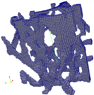
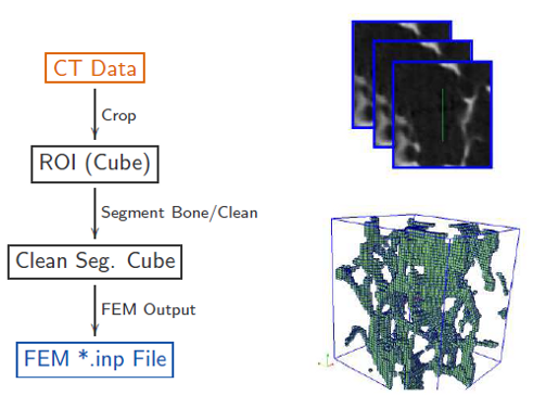
If the ‘temp’ option is not specified, all voxels (except those with GV=0) are converted to FE elements and the same material card is written for all of them. Use ‘.inp’ file format in combination with ‘temp’ option to control which voxel should be converted and which element should get which material card (gray level dependent material). For more details on the format see http://www.calculix.de/
EXAMPLES:
‘.in’ : OOFEM input file format. For details with the ‘temp’ option check the ‘.inp’ file format (above), it uses the same algorithms. For more details on the formats see http://www.oofem.org
‘.fem’ : Altair Optistruct format. All thresholds and bulk material data are written into the fem file. Additionally a density file (‘.sh’) is written. For more details on the formats see http://www.altair.de
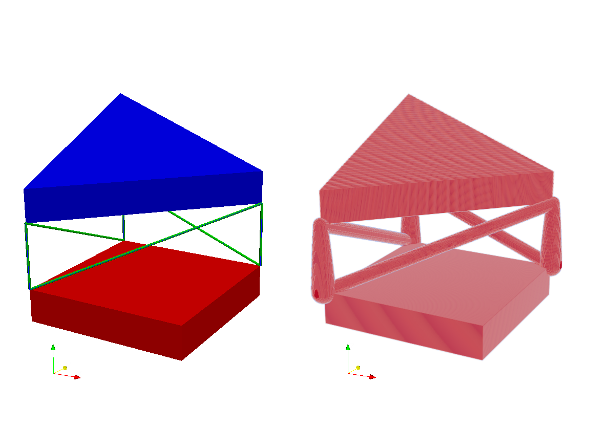
The general idea of FE output is shown in the following Figure:
- -form
: format
Byte format of image file (voxel data) for RAW. Implemented are: B…uint8, H…unit16, h…int16, i…int32, f…float32 Note that the supported format depend on the platform 32 or 64 bit. Depending on the format the file has to be converted to with ‘scale’ option first e.g. for uint8 gray-values from 0-255 are required.
- -zipf
: flag
Compression flag. If flag ‘ON’ compressed files are written in case of ‘mhd’ and ‘nhdr’ file format.
- -mid
: filename
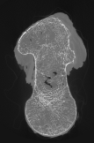
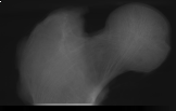
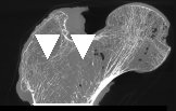
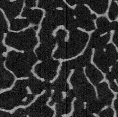
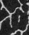
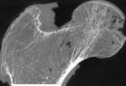
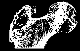
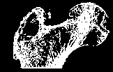
Write mid-plane images of image file (voxel data) in the selected file format. The routine automatically appends “_XM”,”_YM”,”_ZM” at the end of the output file. Available file formats: ‘.png’, ‘.jpg’, ‘.gif’, ‘.tif’, ‘.bmp’, ‘.case’ (Ensight Gold) file format. Additionally the a ‘csv’ file with the ending ‘_INFO’ is written which contains information about the original images.
In addition, a file (ending ‘_INFO.csv’) is written which contains information from the original image from which this image was created. These images and the corresponding information can be displayed in the graphical user interface.
EXAMPLES:
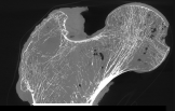
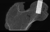
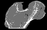
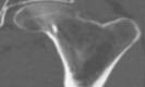
Trabecular bone:


Femur (clinical resolution):
- -proj
: filename
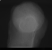
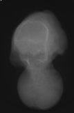
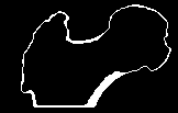
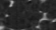
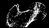
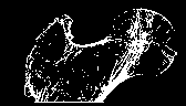
Write projected images of image file (voxel data) in the selected file format. The routine automatically appends “_XP”,”_YP”,”_ZP” at the end of the output file. Available file formats: ‘.png’, ‘.jpg’, ‘.gif’, ‘.tif’, ‘.bmp’. The values are the mean gray values of the projected image. Two corner voxels are set to the minimum and maximum value of the original image.
In addition, a file (ending ‘_INFO.csv’) is written which contains information from the original image from which this image was created. These images and the corresponding information can be displayed in the graphical user interface.
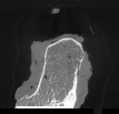
EXAMPLES:
Femur (clinical resolution):
- -mfil
: filter1;;par1;par2;;;filter2;;par3
This option allows to run most of the filters in an arbitrary order. Note that first the active options (filters) are applied on the voxel model. After this run the given filters in this option are applied on the previously modified voxel model. It is recommended do not mix other filters with this option. This means if ‘mfil’ is active, no other options (except ‘Common’) should be active). The option names and default values are the same as for all options implemented in this module. Note: Not all filters are supported with this option.
If you not using the GUI, the different filters are separated by “;;;”. The filter name is separated from the filter parameters with “;;”. The current voxel model is passed to the next filter without storing the results. Use the ‘out’, ‘mid’, etc option to store the results during a multi run in between.
If ‘out’, ‘mid’, ‘proj’ are given than these filters are executed at the end of the multi-run.
- -imr
: startId;step;endId
Image file read parameters. Only needed if image stacks are to be read by given the start, step, and end image number.
The ‘start id’, ‘step’, ‘stop id’ (first, step in, last image number) have to be given. Example: If file0001.png file0003.png file0005.png should be read the format is 1;2;5 and the file name in ‘in’ option should be file####.png (using # as wild card). If single images are read (no wildcards), this option is not needed.
- -raw
: binFormat;headerSize;endianess;fastestDirection
Raw specifiers for reading raw image data (‘.raw’ files).
‘binFormat’: The supported binary format (based on python) like
B   unsigned integer  1 Byte
h   short             2 Byte
H   unsigned short    2 Byte
i   integer           4 Byte
f   float             4 Byte
1   bit               1 Bit (0/1)
‘headerSize’ … size of file header which should be overwritten
‘endianess’ … endian type: ‘big’ or ‘little’
‘fastestDirection’ … fastest varying direction: ‘x’ or ‘z’
- -ldim
: len1;len2;len3
Physical sizes of voxels (length in mm) in 1, 2, 3 direction. Not optional for Abaqus, Vista and Optistruct output! Note that this option influences the physicals units of the FE input files (written by this script).
- -ndim
: nVox1;nVox2;nVox3
Number of voxels in the corresponding 1, 2, 3 direction. Not optional for some input file readers (see ‘in’ option)!
- -temp
: filename
Name of an ABAQUS/Calculix/OOFEM Template file. This option can be used to create an FEA input file from an image. The template file controls the creation of nodes, elements as well as the conversion of gray values to material cards. Internal keywords start with ‘USER’ and are replaced by the script. ABAQUS keywords are copied 1:1 to the created input deck.
Internal supported keywords are:
*USER NODE
  -generate nodes, requires USER PROPERTY keyword
*USER ELEMENT
  -generate elements, requires USER PROPERTY keyword
*USER NSET, type=point, location=arbitrary
  -generate NSET: ARB_NODE_S, ARB_NODE_N, ARB_NODE_E,
                  ARB_NODE_W, ARB_NODE_T, ARB_NODE_B
*USER NSET, type=point, location=addcorner
  -generate NSET: ACOR_NODE_SWB, ACOR_NODE_SEB, ACOR_NODE_NEB,
                  ACOR_NODE_NWB, ACOR_NODE_SWT, ACOR_NODE_SET,
                  ACOR_NODE_NET, ACOR_NODE_NWT
*USER NSET, type=face
  -generate NSET: ALL_NODE_S, ALL_NODE_N, ALL_NODE_E,
                  ALL_NODE_W, ALL_NODE_T, ALL_NODE_B
*USER ELSET, type=face
  -generate ELSET: ALL_ELEM_S, ALL_ELEM_N, ALL_ELEM_E,
                   ALL_ELEM_W, ALL_ELEM_T, ALL_ELEM_B
*USER PROPERTY, file=property_temp.inp, range=minVal:maxVal
  -This line can be repeated multiple times (see example
   below) to created material cards for different
   gray-value ranges. Constant values or Python based
   equations can be given. The variable 'GrayValue' is
   replaced by the gray value of the converted voxel.
  -file= is optional and contains the name of a property
   template file (see second example below).  It could be
   necessary to give also the path to this file.
  -range= gives the gray-value range from minVal till maxVal
   which are are processed i.e. nodes, elements and material
   cards are genereated for the range.  For example, more gray
   values ranges look like 1:69, 70:250, 251:251, 252:255.
   Restriction on ranges: They are not allowed to overlap
   and minVal>0.
  -If the argument 'file=' is not given the property entries
   have to be given directly after the '*USER PROPERTY'
   keyword. At the end of these entries the keyword
   '*USER END PROPERTY' needs to be given.
  -internal variables are for the template file are
   SetName, CardName, GrayValue

Note: _S, _N, _E, _W, _T, _B stands for South, North, East,
West, Top, Bottom). Usually not all *USER NSET and *USER
ELSET keywords are used.
The strings $filename and $pathfilename can be used inside the template file to write the current inp filename without or with the path to the inp file (no extension is written). Only implemented in the case of ABAQUS and CALCULIX.
Example files for CalculiX (similar for Abaqus) are given below. In the first example, the property entries are given directly
** ~~~~~~~~~~~~~~~~~~~~~~~~~~~~~~~~~~~~~~~~~~~~~~~~~~~~~~~~~
** main_temp.inp
** ~~~~~~~~~~~~~~~~~~~~~~~~~~~~~~~~~~~~~~~~~~~~~~~~~~~~~~~~~
*HEADING
main input $filename
** Nodal data from voxel model
*USER NODE
** Elements + elset from voxel model
** type=C3D8, elset="SetName" (see USER PROPERTY)
*USER ELEMENT
** Additional nset from voxel model. New generated nsets are:
** ARB_NODE_S, ARB_NODE_N, ARB_NODE_E, ARB_NODE_W, ARB_NODE_T,
** ARB_NODE_B
*USER NSET, type=point, location=arbitrary
** Additional nset from voxel model. New generated nsets are:
** ACOR_NODE_SWB, ACOR_NODE_SEB, ACOR_NODE_NEB, ACOR_NODE_NWB,
** ACOR_NODE_SWT, ACOR_NODE_SET, ACOR_NODE_NET, ACOR_NODE_NWT
** Note: the nodes are not connected to the model!
*USER NSET, type=point, location=addcorner
** Additional nset from voxel model. New generated nsets are:
** ALL_NODE_S, ALL_NODE_N, ALL_NODE_E, ALL_NODE_W, ALL_NODE_T,
** ALL_NODE_B
*USER NSET, type=face
** Additional elset from voxel model. New generated nsets are:
** ALL_ELEM_S, ALL_ELEM_N, ALL_ELEM_E, ALL_ELEM_W, ALL_ELEM_T,
** ALL_ELEM_B
*USER ELSET, type=face
** User property (section & material) from  template file
** internal variables are: "SetName", "CardName", "GrayValue"
***********************************************************
*USER PROPERTY, range=1:250
*SOLID SECTION, ELSET=SetName, MATERIAL=CardName
1.
*MATERIAL,NAME=CardName
*ELASTIC
5400.*(GrayValue/250.)**2.5, 0.3
*USER END PROPERTY
***********************************************************
*USER PROPERTY, range=251:255
*SOLID SECTION, ELSET=SetName, MATERIAL=CardName
1.
*MATERIAL, NAME=CardName
*ELASTIC
2000., 0.3
*USER END PROPERTY
***********************************************************
*STEP
*STATIC
*BOUNDARY
ALL_NODE_B, 1, 3, 0
*BOUNDARY
ALL_NODE_T, 1, 3, 0.1
*NODE FILE
U
*EL FILE
S
*NODE PRINT, NSET=ALL_NODE_T
RF
*END STEP
** ~~~~~~~~~~~~~~~~~~~~~~~~~~~~~~~~~~~~~~~~~~~~~~~~~~~
In the second case a file ‘property_temp_bone.inp’ and ‘property_temp_embed.inp’ needs to be created additionally
** ~~~~~~~~~~~~~~~~~~~~~~~~~~~~~~~~~~~~~~~~~~~~~~~~~~~~~~~~~
** main_temp.inp
** ~~~~~~~~~~~~~~~~~~~~~~~~~~~~~~~~~~~~~~~~~~~~~~~~~~~~~~~~~
*HEADING
main input $filename
** Nodal data from voxel model
*USER NODE
** Elements + elset from voxel model
** type=C3D8, elset="SetName" (see USER PROPERTY)
*USER ELEMENT
** Additional nset from voxel model. New generated nsets are:
** ARB_NODE_S, ARB_NODE_N, ARB_NODE_E, ARB_NODE_W, ARB_NODE_T,
** ARB_NODE_B
*USER NSET, type=point, location=arbitrary
** Additional nset from voxel model. New generated nsets are:
** ACOR_NODE_SWB, ACOR_NODE_SEB, ACOR_NODE_NEB, ACOR_NODE_NWB,
** ACOR_NODE_SWT, ACOR_NODE_SET, ACOR_NODE_NET, ACOR_NODE_NWT
** Note: the nodes are not connected to the model!
*USER NSET, type=point, location=addcorner
** Additional nset from voxel model. New generated nsets are:
** ALL_NODE_S, ALL_NODE_N, ALL_NODE_E, ALL_NODE_W, ALL_NODE_T,
** ALL_NODE_B
*USER NSET, type=face
** Additional elset from voxel model. New generated nsets are:
** ALL_ELEM_S, ALL_ELEM_N, ALL_ELEM_E, ALL_ELEM_W, ALL_ELEM_T,
** ALL_ELEM_B
*USER ELSET, type=face
** User property (section & material) from  template file
** internal variables are: "SetName", "CardName", "GrayValue"
*USER PROPERTY, file=property_temp_bone.inp, range=1:250
*USER PROPERTY, file=property_temp_embed.inp, range=251:255
***********************************************************
*STEP
*STATIC
*BOUNDARY
ALL_NODE_B, 1, 3, 0
*BOUNDARY
ALL_NODE_T, 1, 3, 0.1
*NODE FILE
U
*EL FILE
S
*NODE PRINT, NSET=ALL_NODE_T
RF
*END STEP
** ~~~~~~~~~~~~~~~~~~~~~~~~~~~~~~~~~~~~~~~~~~~~~~~~~~~
** ~~~~~~~~~~~~~~~~~~~~~~~~~~~~~~~~~~~~~~~~~~~~~~~~~~~
** property_temp_bone.inp
** ~~~~~~~~~~~~~~~~~~~~~~~~~~~~~~~~~~~~~~~~~~~~~~~~~~~
*SOLID SECTION, ELSET=SetName, MATERIAL=CardName
1.
*MATERIAL,NAME=CardName
*ELASTIC
5400.*(GrayValue/250.)**2.5, 0.3
** ~~~~~~~~~~~~~~~~~~~~~~~~~~~~~~~~~~~~~~~~~~~~~~~~~~~
** ~~~~~~~~~~~~~~~~~~~~~~~~~~~~~~~~~~~~~~~~~~~~~~~~~~~
** property_temp_embed.inp
** ~~~~~~~~~~~~~~~~~~~~~~~~~~~~~~~~~~~~~~~~~~~~~~~~~~~
*SOLID SECTION, ELSET=SetName, MATERIAL=CardName
1.
*MATERIAL, NAME=CardName
*ELASTIC
2000., 0.3
** ~~~~~~~~~~~~~~~~~~~~~~~~~~~~~~~~~~~~~~~~~~~~~~~~~~~
- -muscal
: scaleFactor
Scaling factor between the linear attenuation coefficients and the gray-values of the image in case of writing SCANCO ‘.aim’ files. Examples :
Scanco Xtreme CT (AKH Vienna) 8192
Scanco muCT 40 (TU Vienna) 4096
- -smooth
: niter;lambda;kPB;interface;boundary;jacobian
Smooth mesh before output. This filter is only active if Abaqus/Calculix/ParFE grids (meshes) are written. The implementation follows Taubin’s algorithm (see, Taubin, Eurographics 2000, Boyd and Mueller 2006).
‘niter’ is the number of iterations. One iteration means forward (with lambda) and backward smoothing (with mu) smoothing i.e. 2 smoothing steps.
‘lambda’ scaling factor (0<lambda<1)
‘kPB’ pass-band frequency kPB (note kPB=1/lambda+1/mu > 0) => mu
‘interface’ on/off switch for including near interface node smoothing. This option is in the current Fortran code not implemented!!
‘boundary’ boundary smoothing id, have to be provided with
boundary=0 … no smoothing of boundary elements/nodes
boundary=1 … smoothing of boundary elements/nodes but preserving cutting planes
boundary=2 … smoothing of boundary elements/nodes
‘jacobian’ minimal allowed scaled Jacobian. E.g. 0.02 means the smallest allowed volume change is 2% of the initial volume.
EXAMPLES:
- -posmid
: posx;posy;posz
Midplane position. This option extends the output options of the ‘mid’ parameter. By default, the midplanes are taken exactly in the middle of the image. This corresponds to the values
posx, posy, posz = 50., 50., 50.
(given in percent of the image extension
nx, ny, nz). A specific midplane position can be selected by these parameters. For example, the position of the layeriis calculated from (intconverts the value to integer):i = int (posx / 100.0 * (nx-1) + 0.5)
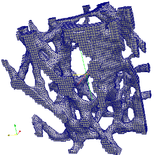
- -mesh2d3
: filename
Write 2D triangular meshes of the interface between gray-values. Only meaningful for segmented voxel models. Use the the ‘smooth’ option to smooth the surface mesh. Possible output formats are:
geom : TAHOE II format
geo : PARAVIEW : Ensight gold format (same as case)
case : PARAVIEW : Ensight gold format (same as geo)
inp : ABAQUS input file
off : Geomview file
msh : GMSH file
EXAMPLES:

- -mesh2d4
: filename
Write 2D quadrilateral meshes of the interface between gray values. Only meaningful for segmented voxel models. Use the the ‘smooth’ option to smooth the surface mesh. Possible output formats are:
geom : TAHOE II format
geo : PARAVIEW : Ensight gold format (same as case)
case : PARAVIEW : Ensight gold format (same as geo)
inp : ABAQUS input file
off : Geomview file
msh : GMSH file
EXAMPLES:
- -sing
: filename;direction;sliceId
Write single images in the selected file format (known by filename extension).
‘filename’ The filename where the routine automatically appends the direction and the slice number (e.g. filname_1+_21.png) at the end of the output file. Available file formats: png, jpg, gif.
‘direction’ The direction (1+,2+,3+,1-,2-,3-) and the slice number in this direction. Positive direction mean one is looking in the direction of the axis.
‘sliceId’ The number of the required slices starting with ‘1’.
- -geom
: type;grayValue;voxelSize;filename;diameter;height
Writes a geometrical object as voxel model to the output. This option ignores the ‘in’ options.
Currently implemented objects are:
sphere : type=’sph’, ‘dim1’=diameter, ‘dim2’ and ‘dim3’ not given
cylinder : type=’cyl’, ‘dim1’=diameter, ‘dim2’=height, ‘dim3’ not given
cube : type=’cube’, ‘dim1’=nx, ‘dim2’=ny, ‘dim3’=nz
The ‘grayValue’ is the voxel gray scale value of the geometrical object. The ‘voxelSize’ is the physical voxel length. The remaining dimensions are given as number of voxels.
- -offs
: off1;off2;off3
Resets the offset off the ‘in’ file to the given values.
- -flip
: axis1;axis2;axis3;…
Flip the model around the given flip axes: The size of the model is not changed.
EXAMPLES:

- -rota
: axi1;axi2;axi3;angle1;angle2;angle3;interpolate
Rotate the voxel model by rotation type ‘angle’:
axi1;axi2;axi3 = Rotation order around axis. For example 3;1;2 means first the model is rotated around 3-axis, second around 1 axis and third around 2 axis
angle1;angle2;angle3 = Rotation angles in Deg around 1,2,3 axis. That means ang1 will be applied in the previous example as second rotation.
interpolate = YES/NO if YES data will be interpolated (preferable)
Note: if the angles are taken from sop.py (Stiffness Optimizer) the model have to be rotated such that rotation order = 1;2;3 and rotation angle = x;y;z (from sop)
Note: The image is increased in size and shifted such that the rotated model fits fully inside. The offset is updated accordingly such that the new image is still in the correct position in the world coordinate system. This can be checked e.g. with Slicer.
EXAMPLES:

- -rotm
: R11;R12;R13;R21;R22;R23;R31;R32;R33;interpolate
Rotate the voxel model by rotation type ‘matrix’:
Rij = coefficients of the rotation matrix
interpolate = YES/NO if YES data will be interpolated (preferable)
Note: The image is increased in size and shifted such that the rotated model fits fully inside. The offset is updated accordingly such that the new image is still in the correct position in the world coordinate system. This can be checked e.g. with Slicer.
- -rotf
: filename;interpolate
Rotate the voxel model by using transformation file. Implemented ‘filename’ can be :
‘tfm’: ITK transformation file. For example, exported from 3D Slicer.
‘nhdr’: NRRD image header file with transformation information in it. The important informations in this file are ‘space directions’ which gives indirectly the transformation matrix and ‘space origin’ which gives the offset.
‘mhd’: ITK meta image header file with transformation information in it. The important informations in this file are ‘TransformMatrix’ which gives the transfromation matrix and ‘Offset’ which gives the offset. The ‘CenterOfRotation’ has to be (0,0,0).
For example, this can the the file given in the ‘in’ option if the applied transformation matrices are inside. More details about the transformation is given in the Mesh - Converter module (fec).
Note: The image is increased in size and shifted such that the rotated model fits fully inside. The offset is updated accordingly such that the new image is still in the correct position in the world coordinate system. This can be checked e.g. with Slicer.
- -mask
: filename
Mask voxel model with the given second voxel model. File have to be segmented and scaled to 0/1 i.e. exactly two gray values (0/1)! Instead the ‘arith’ option can be use to obtain the same results.
EXAMPLES:

- -bool
: operator;filename
Add a second voxel model to the existing one. Compared to ‘arith’ and ‘mask’ the two voxel models do not need to have the same dimensions. The ‘operator’ says how the models are combined. Currently implemented
+,-,*,r(r..replace if gray value larger than 0). If the voxel model is given as ‘mhd’ file, the offset will be taken into account.EXAMPLES:
- -repl
: filename;elset;grayvalue;resolution
Replace the gray-values of a voxel model based on a meshed domain given by ‘filename’. The ‘elset’ is a string of the corresponding element set (name or id) or it can be ‘ALL’ if the whole FE mesh should be used. The ‘grayvalue’ is used for the new gray-value inside the voxel model. If ‘grayvalue’=’None’ than the gray-value is generated from the material IDs starting after the highest grayvalue in the model and steping by one. This function can be used to insert an implant into a bone.
EXAMPLES:
If the ‘resolution’ is given, a new voxel model is generated with zero background and the only the meshed domain is marked. The voxel model given by -out is ignored. It can be used to create a 3D print model from an FE mesh.
EXAMPLES:
The meshed domain have to be given in a format which can be read by the finite elemente converter ‘fec’ (e.g. inp, fem, …).
Linear & quadratic solid elements namely:
tetrahedrons (tetra4, tetra10)
hexahedrons (hexa8, hexa20)
pentahedron (penta6, penta20)
pyramids (pyra5)
lineare structural elements are implemented:
tapered beams (bar2)
triangles (tria3)
quadriliterals (quad4)
In case of structural elements the thickness information is read from the property entry. The beam type can be ‘CIRC’ in case of Abaqus and ‘ROD’ in case of Optistruct. If elements are outside the given voxel model a warning will be thrown.
- -arith
: operation1;operation2;…
Apply an equation/formula on the data array. Implemented operators are:
+A  ... add value A to loaded voxelmodel
-A  ... subtract value A from loaded voxelmodel
*A  ... multiply with A
/A  ... divide by A
<B  ... store current value in B
>B  ... load B in current value
^I  ... power I (only integers!) of current value
>>C ... load file with name C into memory (mhd, nhdr, or isq)
?   ... logical conditions like ?<0=0 or ?==3=2 or ?>7=12
&sin ... compute sinus of array in memory
&cos ... compute cosinus of array in memory
&arcsin ... compute arcus sinus of array in memory
&arccos ... compute arcus cosinus of array in memory
&tan    ... compute tangens of array in memory
&arctan ... compute arcus tangens of array in memory
EXAMPLES:

- -labvox
: outValue;roiValue;n0Vox1;n0Vox2;n0Vox3;dnVox1;dnVox2;dnVox3
Labels a small part of a bigger model with ‘roiValue’. The sourrounding voxels have ‘outValue’. If ‘outValue’=None, the value of the input image is used.
The region is defined by using start voxel ids (‘n0Vox1’, ‘n0Vox2’, ‘n0Vox3’) and the size of a ROI (‘dnVox1’, ‘dnVox2’, ‘dnVox3’).
Alternatively, the keyword ‘cube’ can be added (9 entries), so the entry shows:
outValue;roiValue;n0Vox1;n0Vox2;n0Vox3;dnVox1;dnVox2;dnVox3;cube
In this case ‘n0Vox1;n0Vox2;n0Vox3’ are the center of cube and ‘dnVox1;dnVox2;dnVox3’ is the size of the cube.
EXAMPLES:

- -scale
: newMin;newMax;oldMin;oldMax;format
Scale the min/max values of a voxel model. If old values (PARAM “oldMin;oldMax”) are not given the min and max values of the original voxel model will taken instead of given values. The string ‘oldMin’ or ‘oldMax’ can be used in old or new values. (Example oldMin;255;70;oldMax). If the format specifier is given the return format of the filter can be controlled. The default format is the input format of the voxel array.
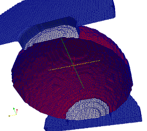
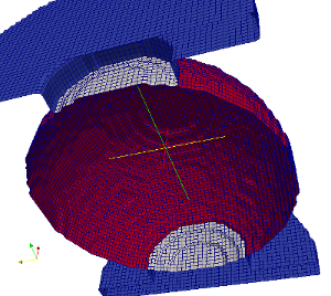
- -fill
: threshold;valid;type;kernel;[minThick];[niter];[kernel2];[bx0]; [bx1];[by0];[by1];[bz0];[bz1]
Fill the pores of a segmented image. Details can be found in : Pahr and Zysset, Comput Methods Biomech Biomed Engin, 2009, 12, 45-57 Parameters are described in this paper and are:
‘threshold’ the threshold value which is used to segment the image
‘valid’ is also some kind of a threshold. The algorithm counts how often a voxel was marked as a fill voxel. Maximum marks are seven. E.g. ‘valid’=5 means that also voxels which are five times marked are treated as fill voxels.
‘type’ gives the type of the algorithm. Implemented options are:
out … outer surface (param1 = smooth)
in … inner surface (param1 = smooth)
t … cortical shell (param1 = smooth)
- v … value from filling (for test purposes!)
(param1 = smooth)
c … contour of filling (thickness is given by min_t)
Add ‘_2d?’ with ?=1,2,3 if 2D filling should be selected. The “?” gives the direction of the normal of the 2D plane. E.g. ‘out_2d3’ means outer surface fill in 2D where the 3-axis is normal to this plane. If ‘_2d?’ is not given the 3d search option is used as default.
‘kernel’ : size (radius) of smooth kernel in voxels dimensions
‘minthick’: optional - minimal cortex thickness, only used in ‘type’=c
‘niter’ : optional - maximum number of fill error correction iterations. If not given or set to 0 no correction will be done.
‘kernel2’: optional -size (radius) of kernel in voxels for the fill error correction steps. If not given it is the same as “kernel”.
‘bx0;bx1;by0;by1;bz0;bz1’ : optional - bounding box which is used to apply the fill error correction.
EXAMPLES:
Thickness:
Outside (with 2d3, without):


Outside with correction (full, bounding box):


- -cont
: threshold
Extracts the contour based on the given threshold. All voxels >= threshold will be included in the evaluation. Edges and corners are not implemented in the contour search.
EXAMPLES:

- -distt
: None
Distance transform based on Saito Method. A binary input input image is required. The distance tansform is computed on the “white” part.


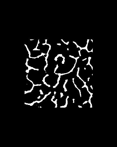
- -skel
: None
Compute the skeleton of a binary image.
- -sitkf
: filename
This filter allows to execute Simple ITK code which is located in ‘filename’. The two variable names ‘sitkInputImage’ and ‘sitkOutputImage’ are reserved for the input image and the output image, respectively. Example file content
sitkOutputImage = sitk.BinaryThreshold(sitkInputImage,
                   lowerThreshold=100,
                   upperThreshold=200,
                   insideValue=255,
                   outsideValue=0)
An ‘import SimpleITK as sitk’ is done automatically by medtool.
Fixed parameters of the function can be replaced by variable by using the ‘sitkp’ option.
An other example with image recasting is the BinaryThinning
binaryImage = sitk.Cast(sitkInputImage, sitk.sitkUInt8)
sitkOutputImage = sitk.BinaryThinning(binaryImage)
sitkOutputImage = sitk.PermuteAxes(sitkInputImage, order=[2,0,1])
- -sitkp
: If the option ‘sitkf’ is active, you can use this option to pass variables to a simple ITK filter.
The variable names are freely selectable. The following data types are detected automatically :
integer : ‘-1’, ‘200’
float : ‘2.35’
lists : ‘20;30;40’
strings : ‘filename.mhd’
Example (regions growing filter)
sitkOutputImage = sitk.ConnectedThreshold(sitkInputImage,
                   seedList=[seed1,seed2],
                   lower=lower,
                   upper=upper,
                   replaceValue=replaceValue)
where, for example, the following entries are required in medtool
seed1        | 20;34;89
seed2        | 56;95;101
lower        | 0
upper        | 1
replacevalue | 1
- -laham
: weight;cutoff;amplitude
Laplace-hamming filter: Transfers image to the frequency domain and
applies the laplace operator
weights the laplacian filtered image with parameter ‘weight’
multiplies the original image with 1-‘weight’
sum up both images
multiplies the resulting image with a low pass filter.
The low pass filter follows the formula ampl=’amplitude’
A(k) = (1-ampl/2) - ampl/2*cos(2*pi*k/(M*cutoff-1))
Some characteristics are:
ampl = 0 no low pass filtering is done
ampl = 1 and cutoff=0 … Hanning filter
ampl = 0.92 and cutoff=0 … Hamming filter
where
cutoff*Nyquist_frequency = cut_off_frequency
Note thatboth parameters are ratios and have to be between 0..1.
EXAMPLES:

- -sobel
: None
Sobel filter (only a dummy argument is required but not used). This is a classical edge detection filter
EXAMPLES:

- -mean
: kernel;thres1;thres2
Mean filter: ‘kernel’ gives the type of the kernel window. Only voxels with a gray value >= ‘thres1’ and value <= ‘thres2’ are considered in the computations.
Possible values for ‘kernel’ are :
‘kernel’ is a specifier of following type:
“k3x3”, “k5x5”, “k7x7”, … which is a squared kernel window of size 3x3, 5x5, … where the numbers have to be odd numbers which are seperated by an ‘x’.
“k6”: This is a 3x3 kernel with 6 non-zero values. This is the same as “k1.0”.
“k18”: This is a 3x3 kernel with 18 non-zero values. This is the same as “k1.732” (<sqrt(3)).
“k?.??” where ?.?? is an abitrary float number > 1.0. This number is the radius of a sphere in voxel dimensions which will set up the non-zeros in the kernel window. It is important to write ‘.’ as decimal point. Examples are ‘kernel’=”k1.0”, ‘kernel’=”k2.34”, …
‘kernel’ = number e.g. ‘kernel’=3. In this case the size of the kernel window in voxel dimensions is n = int(2*(‘kernel’+0.5)).
The kernel window is cropped by the bounding box of the image.
EXAMPLES:

- -median
: kernel;thres1;thres2
Median filter: ‘kernel’ gives the type of the kernel window. Only voxels with a gray value >= ‘thres1’ and value <= ‘thres2’ are considered in the computations.
Possible values for ‘kernel’ are :
‘kernel’ is a specifier of following type:
“k3x3”, “k5x5”, “k7x7”, … which is a squared kernel window of size 3x3, 5x5, … where the numbers have to be odd numbers which are seperated by an ‘x’.
“k6”: This is a 3x3 kernel with 6 non-zero values. This is the same as “k1.0”.
“k18”: This is a 3x3 kernel with 18 non-zero values. This is the same as “k1.732” (<sqrt(3)).
“k?.??” where ?.?? is an abitrary float number > 1.0. This number is the radius of a sphere in voxel dimensions which will set up the non-zeros in the kernel window. It is important to write ‘.’ as decimal point. Examples are ‘kernel’=”k1.0”, ‘kernel’=”k2.34”, …
The kernel window is cropped by the bounding box of the image.
EXAMPLES:


- -gauss
: radius;sigma;thres1;thres2
Gaussian filter: Filter computes the Gaussian smoothing of all voxels around a considered voxel within the ‘radius’ by using ‘sigma’. Only voxel with a value >= ‘thres1’ and value <= ‘thres2’ are considered.
EXAMPLES:

- -morph
: radius;type;shape;thres
Morhological filters: compute morphological opening (“o”), closing (“c”), erosion (“e”), dilation (“d”). Similar to ‘morpk’ but with different kernel definitions. Parameters are:
‘radius’ is a radius of specifying the kernel (in number of voxels). The size of the kernel is nk = int(2*(r+0.5)). This means that a radius of “1” gives a kernel of 3x3x3 voxels. In case of a spherical kernel everything which is inside rc <= nk/2 is taken as kernel.
‘type’ specifies if opening (dilation + erosion) or closing (erosion+dilation), or erosion or dilation will be performed.
‘shape’ specifies if a rectangle (“1”) or spherical kernel shape (“2”) should be used.
‘threshold’ is a value which is used to segment the image before applying the filters
EXAMPLES:
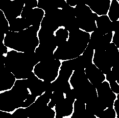
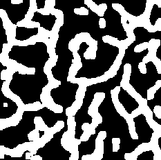
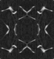
Original Images:
Opening / Closing:


Erosion / Dilation
- -morpk
: kernel;type;thres
Morhological filters: compute morphological opening (“o”), closing (“c”), erosion (“e”), dilation (“d”). Similar to ‘morph’ but with different kernel definitions. Parameters are:
‘kernel’ is a specifier of following type:
“k3x3”, “k5x5”, “k7x7”, … which is a squared kernel window of size 3x3, 5x5, … where the numbers have to be odd numbers which are seperated by an ‘x’.
“k6”: This is a 3x3 kernel with 6 non-zero values. This is the same as “k1.0”.
“k18”: This is a 3x3 kernel with 18 non-zero values. This is the same as “k1.732” (<sqrt(3)).
“k?.??” where ?.?? is an abitrary float number > 1.0. This number is the radius of a sphere in voxel dimensions which will set up the non-zeros in the kernel window. It is important to write ‘.’ as decimal point. Examples are ‘kernel’=”k1.0”, ‘kernel’=”k2.34”, …
- ‘type’ is the type of the morphological operation. It can
be ‘o’, ‘c’, ‘e’, or ‘d’.
‘thres’ is a value which is used to segment the image before applying the filters
- -grad
: None
Gradient filter (only dummy argument required - not used).
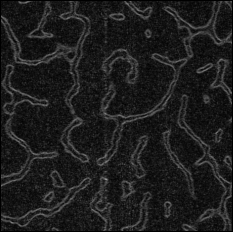
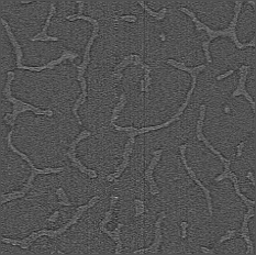
EXAMPLES:
- -lapl
: None
Laplacian filter (only dummy argument required - not used).
EXAMPLES:
- -avg
: filename;phyWinSize;thres;maskValue
The function averages gray value over a ROI with a size of ‘phyWinSize’ in mm and writes the results to a file ‘filename’.
The algorithm starts at the physical 0/0/0 location and steps over the images with a distance of ‘phyWindowSize’ (cube). It selects all voxels which have there COG inside the window. If a ‘thres’=’None’ average gray value are computed and the output variables (written in ‘filename’) are
nx0;ny0;nz0;dnx;dny;dnz;lx;ly;lz;ZV;TV;grayValueAverage
otherwise ‘threshold’=somevalue
nx0;ny0;nz0;dnx;dny;dnz;lx;ly;lz;ZV;TV;BVTV
If the ‘maskValue’ is given (not =’None’) it will be considered in the computations of the average. Voxels with a gray value of ‘maskValue’ are not part of the ROI. For example, in case of density computations this means
BVTV = BV/(TV-ZV)
where ZV is equal to the ‘maskValue’.
- -cfill
: nlevels
Octree based filling of a segmented voxel model. A voxel model with a single threshold (e.g. 0 and 75) has to be provided. The filter colors depending on the given ‘nlevels’ cubes of size 2*1, 2*2, … 2*nlevels. The lower level has the gray value nlevels+1, the highest has a grayvalue of 1.
EXAMPLES:
- -cut
: n0Vox1;n0Vox2;n0Vox3;dnVox1;dnVox2;dnVox3
Cut/crop a small part of a bigger model by using start voxel ids (‘n0Vox1’, ‘n0Vox2’, ‘n0Vox3’) and the size of a ROI (‘dnVox1’, ‘dnVox2’, ‘dnVox3’). This size will be the new size of the voxel model. i.e. three positions of the new origin (old origin at 0;0;0) and three extensions (number of voxels) = ROI.
EXAMPLES:
- -bbcut
: threshold;extVox1;extVox2;extVox3
Cut/crop a small part of a bigger model by using an automatic bounding box search algorithm. The bounding box is detected using the ‘threshold’. The three optional values ‘extVox1’, ‘extVox2’, ‘extVox3’ are the number of voxels in 1, 2, 3 which should increase the bounding in all directions
EXAMPLES:
- -roicut
: x0;y0;z0;x1;y1;z1
Cut/crop a small part of a bigger model by using a ROI given in physical dimensions. ‘x0’, y0’, ‘z0’ are the start coordinates and ‘x1’, y1’, ‘z1’ are the end coordinates the the bounding box of the ROI. Note the “one voxel” inaccuracy due to this method.
If the image data contain an offset (‘mhd’ or ‘nhdr’) it is taken into account.
- -roitxt
: filename.txt
Cut/crop a small part of a bigger model by using a ROI given in physical dimensions. Compared to the ‘roicut’ option, the ROI dimensions are read from a text file. Note the “one voxel” inaccuracy due to this method.
If the image data contain an offset (‘mhd’ or ‘nhdr’) it is taken into account.
- -mcut
: dnVox1;dnVox2;dnVox3
Cut/crop a ROI from the middle of a bigger voxel model. Teh size of the model is given by the three extensions ‘dnVox1’, ‘dnVox2’, ‘dnVox3’ (number of voxels in 1,2,3).
EXAMPLES:

- -res2
: res1;res2;res3
Change the resolution of the voxel data. ‘res1;res2;res3’ are the new resolutions (voxel model size) in 1,2,3 axis.
Avoid the usage of this filter because it is slow and interpolates voxel data. ‘resf’ is recommended.
- -res3
: len1;len2;len3
Change the resolution of the voxel data by given voxel lengths. ‘len1;len2;len3’ are approximations of the new voxel lengths. They are adopted such that the voxel model size will be unchanged.
Avoid the usage of this filter because it is slow and interpolates voxel data. ‘resf’ is recommended.
- -res4
: len1;len2;len3
Change the resolution of the voxel data by given voxel lengths. ‘len1;len2;len3’ are the exact the new voxel lengths. The voxel model size (nx, ny, nz) is adopted accordingly.
Avoid the usage of this filter because it is slow and interpolates voxel data. ‘resf’ is recommended.
- -resf
: factor
Change the resolution (recoarse/refine) of the voxel data by the given ‘factor’. Note that the overall size of the voxel model might change slightly in case of recoarsening because no interpolations is done.
Positive ‘factor’ values recoarse the image, negative ‘factor’ values refine the image by this factor.
EXAMPLES:

- -refi
: direction;factor
Refine the image in one direction (given by ‘direction’ either 1,2, or 3) by a given factor. This filter can be used to convert anisotropic QCT images to isotropic once.
EXAMPLES:
- -mirr
: axis1;axis2;axis3;…
Mirror the model around the given mirror axes. The size of the model is doubled in the given direction.
EXAMPLES:
- -mir2
: nVox1;nVox2;nVox3
Mirror the model such that it fills a new array with dimension ‘nVox1’, ‘nVox2’, ‘nVox3’. This filter is used to create arrays for FFT.
EXAMPLES:

- -autot
: BVTV;error;estimate
Find the threshold for a given ‘BVTV’ value within a given ‘error’. In order to increase speed an threshold ‘estimate’ should also be given. All voxels below the computed threshold will be set to the lowest value in the model. The rest (the object) will be given to the computed value.
- -fixt
: thresRatio;minimum;maximum
The image is binarize by using this command. A fixed threshold is applied on the image. The given parameter ‘thresRatio’ is a ratio for the computations (see example below). The second and third parameter specifies the ‘minimum’ and ‘maximum’ range of the threshold. Allowed values numbers as well as strings like ‘minVal’ and ‘maxVal’. In this case these values are computed from the image. Example (thresRatio=0.4, minVal = -100, maxVal = 2000)
0.4;minVal;maxVal -> threshold = (2000-(-100))*0.4
0.4;0.0;maxVal    -> threshold = (2000-0.0)*0.4
0.4;0.0;200       -> threshold = (200-0.0)*0.4
This method is suggested in the literature to segment HR-pQCT images.
- -slevt
: startValue
The image is binarize by using the method of Ridler. The threshold is computed iteratively using a single level thresholding. The given ‘startValue’ is used to decide which values should be considered during the computation. For example, if ‘startValue’ is 1, all values below 1 are not included in the computations.
The thresholding technique described in ‘thre0’ is used for segmentation. All voxels below the computed value will be set to the value 0, the rest (the object) will be set to the computed value.
This is the recommended segmentation option for high-resolution micro-CT images.
EXAMPLES:
- -dlevt
: thres1;thres2
The image is binarize by using the method of Ridler. The threshold is computed iteratively using a double level thresholding. The function is simular to ‘slevt’ but two threshold values are computed. The given search thresholds ‘thres1’ and ‘thres2’ should be chosen properly.
The thresholding technique described in ‘thres’ is used for segmentation. All voxels below the computed value will be set to the lowest gray-value, the rest (the object) will be set to the computed values.
EXAMPLES:
- -rthres
: lower;upper;thres
An image is binarize by using this command. All voxels below ‘lower’ and above ‘upper’ will be set to the value 0, the rest (the object) will be given a value of ‘thres’.
- -lthres
: type;alpha;LT;UT
Binarize the image by using a local adaptive threshold computed from local measures of the image. The kernel is a 3x3x3 cube. Parameters are:
‘type’ : “stddev”: similar to the method proposed by Kang and Engelke 2003. The criterion is
voxValue < (mean-alpha*stddev) --> marrow voxel
where voxValue is the grayvalue of the cube’s center, mean and stddev (n-1) is computed from the kernel.
‘alpha’ : This is the scaling for the weighting
- ‘LT’lower threshold. Everything below is marrow. If not
given the threshold is automatically estimated by the mean grayvalue (same as -mthres).
‘UT’ : upper threshold. Everything above is bone. If not given the threshold is automatically estimated by the histogram (same as -slevt).
All voxels below the computed value will be set to the value 0, the rest (the object) will be set to 1.
EXAMPLES:

- -gthres
: type
Binarize the image by using a global threshold computed from global measures of the image. ‘type’ can be either “mean” or “median”.
All voxels below the computed value will be set to a value of 0, the rest (the object) will be set to the computed threshold value.
EXAMPLES :
- -thres
: thres1;thres2;…
Binarize the image by using one or more thresholds ‘thres1’, ‘thres2’, … The first threshold has to be bigger or equal to the lowest gray value in the model.
Everything below ‘thres1’ is set to the lowest gray-value found in the image. For example, for a 25;75 threshold list, all values below 25 will be set to lowest value found in the image. All voxel ranging from 25 to 74 will be set to 25 and all voxel above 75 will be set to 75.
Note: Only grayvalue>0 will produce an FEM element (if inp file is selected in ‘out’ option). Use the option ‘thre0’ to avoid these issues.
EXAMPLES : Original / 1 Threshold / 2 Thresholds


- -thre0
: ‘threshold’
Binarize the image by using a single ‘threshold’ value. Compared to the ‘thres’ option, this option needs only one ‘threshold’ value.
All voxels below the computed value will be set to a value of 0, the rest (the object) will be set to ‘threshold’.
- -clean
: type
This option cleans the segmented (binary) image file which contains ‘0’ and values >’0’. Different variations are implemented:
‘type’ = ‘FAST’: Delete unconnected regions of ‘bone’ material (gray value > 0). The background gray value (air) has to be ‘0’.
‘type’ = ‘FAST1’: Delete unconnected regions of ‘air’ material (gray value = 0).
‘type’ = ‘FAST2’: Runs option ‘FAST’ (delete unconnected ‘bone’ regions) followed by ‘FAST1’ (delete unconnected regions of ‘air’ material with gray value = 0).
‘type’ = nodes;island: Similar to first possibility (‘FAST’) but much slower. The first variable (‘nodes’) is the minimum number of shared nodes between connected bone region of deletion algorithm. The second value (‘island’) is a minimum number of bone/marrow voxels. If an island is detected with less voxels, it is deleted.
‘type’ = ‘NUMPY’: Delete unconnected regions of foreground voxels. Only two different materials are allowed. The bg has not to be 0.
‘type’ = ‘NUMPY1’: Delete unconnected regions of background voxels. Only two different materials are allowed. The bg has not to be 0.
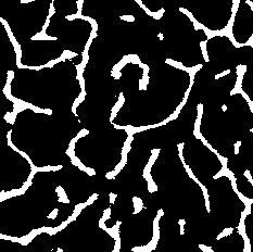
EXAMPLES : Original / Clean (‘FAST’)
EXAMPLES : Original / Clean (‘FAST1’)


- -extend
: direction;thickVox;[newGrayvalue]
Extend the model. Following parameters are required:
‘direction’ is the direction of embedding. It can be -1 (x=0), 1 (x=nx), -2 (y=0), 2 (y=ny), -3 (z=0), 3 (z=nz).
‘thickVox’ is the number of extended voxel layers (thickness).
‘newGrayvalue’ (optional) is a new grayvalue for the extended material. If the thisparamater is given the extended region has not the original grayvalue but this one. Only the voxels with a grayvalue bigger than 0 are modified.
EXAMPLES : Original / Threshold + Extended

- -close
: direction;threshold;kernel;newGrayValue
Close open models at the boundary. Parameters are:
‘direction’ gives the direction of closing. It can be 1 (x), 2 (y), or 3 (z).
‘threshold’ and ‘kernel’ are parameters which are used to close the slice (see ‘fill’ option for details).
‘newGrayValue’ gives the gray value which should be used for the new fill voxels.
The new model will not change in size, only the first and last layer will be replaced.
EXAMPLES :
- -embed
: direction;thickVoxIn;thickVoxOut;newGrayValue
Embed model in a new material. Parameters are:
‘direction’ gives the direction of embedding (1,2,3). You can use + or - to indicate embed on top (+) or bottom (-) only. If no sign is given, both directions will be embedded.
‘thickVoxIn’ and ‘thickVoxOut’ give the thickness of the embedding layer inside and outside of a bounding box (number of voxels). Inside voxels with a value of “0” and all outside voxel will be set to ‘newGrayValue’.
EXAMPLES : 3- / 3+ / 2- / 2+


- -cap
: direction;thickVox;newGrayValue
Make an end cap (bone material) on both ends in given direction of given thickness (number of voxels). The voxels will set to the given gray value. Parameters are:
‘direction’ gives the direction of embedding (1,2,3). You can use + or - to indicate embed on top (+) or bottom (-) only. If no sign is given, both directions will be embedded.
‘thickVox’ is the thickness of the cap
‘newGrayvalue’ gray-value of the generated voxels.
EXAMPLES :

- -cover
: thickVox;newGrayValue
Surround the whole model with a layer of material with given thickness (number of voxels). Parameters are:
‘thickVox’ thickness of the cover voxels.
‘newGrayValue’ gray-value of the generated voxels.
EXAMPLES :

- -block
: nVox1;nVox2;nVox3;newGrayValue
Place the voxel model inside a bigger block of material. Parameters are:
‘nVox1’, ‘nVox2’, ‘nVox3’ which are the number of voxels in 1,2,3 direction of the new block
‘newGrayValue’ is the gray-value background of the new block
EXAMPLES :
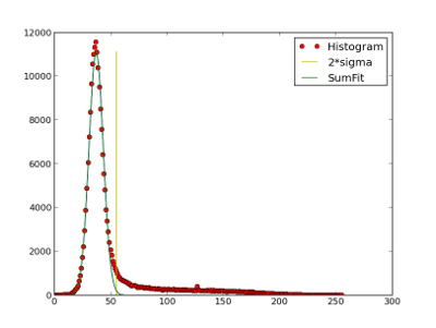
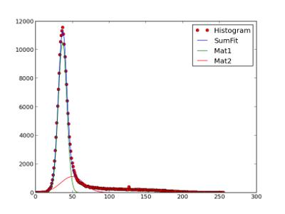
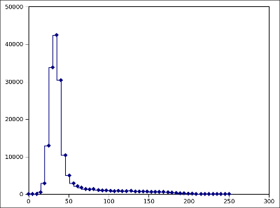
- -shist
: type;[filename];[mode]
‘type’ = 0 shows a histogram of the image data including the mean and standard deviation of the data. The parameters ‘filename’ and ‘mode’ are ignored by this option. The histogram data can be output to a file with the option ‘histo’.
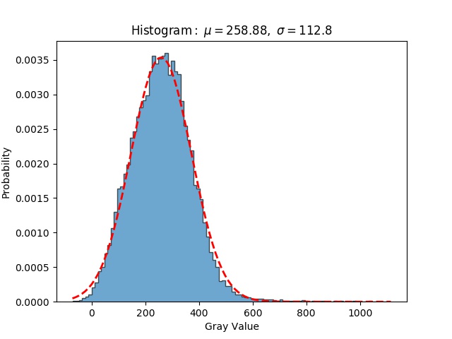
‘type’=1,2,3 fits one, two or three bell-shaped distributions through the histogram data. In this way, the gray scale distribution of bone marrow and bone can be simulated. The gray-value histogram and fitted data are shown. Further parameters for these three types are:
‘filename’ (optional) where the computed coefficients of the fitted function are given.
‘mode’ of writing (python style) can be:
‘w’ (create new file) write header + data) and
‘a’ (append to file, write data).
This option shows a histogram using matplotlib e.g. fit 1 or 2:
- -histo
: filename;normalize;nIntervals
Output histogram data in a file.
‘filename’ where the computed info is written.
‘normalize’ option. Can only have the values ‘y’ or ‘n’. If ‘y’ the percentage of volume within the interval instead of the number of voxel will be given.
‘nIntervals’ number of intervals, if not given, the interval size will be “1”.
It writes data to a file which can be plotted with Excel e.g.:
- -cen
: threshold;filename;mode Compute the first voxel near center which has a value bigger or equal than the given ‘threshold’. It also computes the radius of a sphere located in this point which captured the full voxel model. This values are needed by the CGAL surface mesher. The output is in physical dimensions which is written to ‘filename’ using ‘mode’. In detail:
‘filename’ If given the computed info is written into the file.
‘mode’ of writing (python style) can be:
‘w’ (create new file) write header + data) and
‘a’ (append to file, write data).
- -bbox
: type;threshold;filename;mode;i;j;k
Writes a bounding box to a given filename. Parameters are:
‘type’ can be “in” for inside or “out” for outside.
‘threshold’ is the given to indicate the boundary of the box.
‘filename’ where the computed info is written.
‘mode’ of writing (python style) can be:
‘w’ (create new file) write header + data) and
‘a’ (append to file, write data).
- ‘i,j,k’ are the starting points i,j,k of the search is
used only in the “in” bounding box. If it is not given the middle of the voxel model will be used.
Note: For the inner bounding box the model has to be enclosed by matter.
It writes following info to a file:
#filename;threshold;bbType;minX;minY;minZ;maxX;maxY;maxZ
femur-r8.mhd;100;in;0;0;0;106;161;102
- -cog
: newGrayValue
Compute the center of gravity. There will be an output on the screen and if activagted in the information file (‘ifo’). The parameter ‘newGrayValue’ is a gray value which is be used to plot the 3 orthogonal planes indicating the cog in the voxel model. If ‘newGrayValue’ = ‘off’ the planes are not plotted in the voxel file.
- -ifo
: filename;mode
Write general information to a file. This option can be very helpful to generate a CSV file from your dataset.
‘filename’ where the computed info is written.
‘mode’ of writing (python style) can be:
‘w’ (create new file) write header + data) and
‘a’ (append to file, write data).
It writes following CSV table to a file:

- -sifo
: filename;mode;preName;val1;val2; ….
Write specific information to a file. This option can be very helpful to generate a CSV file from your dataset.
‘filename’ where the computed info is written.
‘mode’ of writing (python style) can be:
‘w’ (create new file) write header + data) and
‘a’ (append to file, write data).
- ‘preName’ String which is added before the variable name,
e.g. ‘$’, ‘VAL’, or ‘’ (empty string)
‘val1’, ‘val2’, … are implemented keys which are:
‘VOI_DimSize_x’, ‘VOI_DimSize_y’, ‘VOI_DimSize_z’ (= nx, ny, nz)
‘VOI_ElementSpacing_x’, ‘VOI_ElementSpacing_y’, ‘VOI_ElementSpacing_z’ (= lx, ly, lz)
‘VOI_Size_x’, ‘VOI_Size_y’, ‘VOI_Size_z’ (= nx*lx, ny*ly, nz*lz)
‘VOI_Offset_x’, ‘VOI_Offset_y’, ‘VOI_Offset_z’
‘minVal’, ‘maxVal’
‘voxSum’, ‘graySum’
‘greaterZeroSum’ (number of voxels with a value > 0
‘grayAvg’ = ‘graySum’/’voxSum’
‘greaterZeroGrayAvg’ = ‘graySum’/’greaterZeroSum’
It writes following CSV table to a file:
Write general information to a file. This option can be very helpful to generate a CSV file from your dataset.
‘filename’ where the computed info is written.
‘mode’ of writing (python style) can be:
‘w’ (create new file) write header + data) and
‘a’ (append to file, write data).
It writes following CSV table to a file:
- -help
: Print usage
Info
File: mic.py
Author: D.H. Pahr
Processor (MPI)
This module is a parallel extension of medtool’s Image-Processor script (mic) and contains selected 3d image processing algorithms of the mic version. It takes 3d medical CT image data sets (voxel models) as input and creates new, modified image data.
The scripts can be run with single or multiple CPUs. The speed-up is high as long as the given number of CPUs is lower or equal to the physical available number of CPUs on the used machine.
The input image is passed as memory-map. Memory-maps are ideal for accessing small segments of large files on disk. In combination with multiple CPUs the scripts is fast and shows a low memory requirement.
If multiple processing steps are combined, numpy arrays (no memmaps) are created internally which increases the memory requirement. To keep the memory imprint as low as possible, write out the files immediately after the first run. Compared to the mic model, the output and input data types are unchanged if no floating point computations are done with the data.
Usage
Module:
import mic_mpi
Command line:
python mic_mpi.py ...

  -in       filename
  [-out]    filename                                          [optional]
  [-form]   format                                            [optional]
  [-mid]    filename                                          [optional]
  [-arith]  operation1;operation2;...                         [optional]
  [-scale]  newMin;newMax;[oldMin];[oldMax];[format]          [optional]
  [-morpk]  kernel;type;thres                                 [optional]
  [-cut]    n0Vox1;n0Vox2;n0Vox3;dnVox1;dnVox2;dnVox3         [optional]
  [-roicut] x0;y0;z0;x1;y1;z1                                 [optional]
  [-resf]   factor                                            [optional]
  [-thres]  thres1;thres2;thres3;...                          [optional]
  [-np]     value                                             [optional]
  [-memmap] flag                                              [optional]
  [-block]  value                                             [optional]
  [-mfil]   filter1;;par1;par2;;;filter2;;par3                [optional]
Parameters
- -in
: filename
The image data file (voxel data). The file type is recognized by the file extension. Possible extensions are:
‘.mhd’ : MetaImage file(ITK). Consist of a meta data file ‘.mhd’ and a binary ‘.raw’ file. The mhd file contains all important informations. It is readable by a text editor. The data itself are stored in a separate raw file. This or the ‘.nhdr’ is the recommended file format.
‘.nhdr’ : NRRD image file composed of a header ‘.nhdr’ and a binary ‘.raw’ file like the mhd format. This is the recommended file format if transformations are important and Slicer3D is used.
‘.isq’ : SCANCO ‘isq’ file format (primary format of SCANCO scanners)
These types consist of a meta data information and raw data sections. This style is necessary for memory-maps.
- -out
: filename
Write image file (voxel data) to a new file. Use the ‘form’ option to control the data type of a singe voxel. Otherwise the format will be chosen depending on the used filter. The file type is recognized by the file extension. Possible file formats are (see ):
‘.mhd’ : ITK meta image file composed of a header and raw data file.
‘.nhdr’ : NRRD image file composed of a header and raw data file.
‘.aim’ : SCANCO ‘aim’ file.
‘.png/.jpg/.gif/.tif/.bmp’ : Single or Stack of image files.
‘.bin’ : ISOSURF file format.
‘.raw’ : Standard binary raw file.
‘.inr.gz’ : Inria image format. Binary file with header in gzip format.
‘.svx’ : Shapeways file format for 3D printing
- -form
: format
Byte format of image file (voxel data) for RAW. Currently implemented B…uint8, H…unit16, h…int16, i…int32, f…float32 Note that the supported format depend on the platform 32 or 64 bit. Depending on the format the file has to be converted to with ‘scale’ option first e.g. for uint8 gray-values from 0-255 are required.
- -mid
: filename
Write mid-plane images of image file (voxel data) in the selected file format. The routine automatically appends “_XM”,”_YM”,”_ZM” at the end of the output file. Available file formats: ‘.png’, ‘.jpg’, ‘.gif’, ‘.tif’, ‘.bmp’, ‘.case’ (Ensight Gold) file format.
- -arith
: operation1;operation2;…
Apply an equation/formula on the data array. Implemented operators are:
+A  ... add value A to loaded voxelmodel
-A  ... subtract value A from loaded voxelmodel
*A  ... multiply with A
/A  ... divide by A
<B  ... store current value in B
>B  ... load B in current value
^I  ... power I (only integers!) of current value
>>C ... load file with name C into memory (mhd, nhdr, or isq)
?   ... logical conditions like ?<0=0 or ?==3=2 or ?>7=12
&sin ... compute sinus of array in memory
&cos ... compute cosinus of array in memory
&arcsin ... compute arcus sinus of array in memory
&arccos ... compute arcus cosinus of array in memory
&tan    ... compute tangens of array in memory
&arctan ... compute arcus tangens of array in memory
EXAMPLES:
- -scale
: newMin;newMax;oldMin;oldMax
Scale the min/max values of a voxel model. If old values (PARAM “oldMin;oldMax”) are not given the min and max values of the original voxel model will taken instead of given values. The string ‘oldMin’ or ‘oldMax’ can be used in old or new values. (Example oldMin;255;70;oldMax).
- -morpk
: kernel;type;thres
Morhological filters: compute morphological opening (“o”), closing (“c”), erosion (“e”), dilation (“d”). Parameters are:
‘kernel’ is a specifier of following type:
“k3x3”, “k5x5”, “k7x7”, … which is a squared kernel window of size 3x3, 5x5, … where the numbers have to be odd numbers which are seperated by an ‘x’.
“k6”: This is a 3x3 kernel with 6 non-zero values. This is the same as “k1.0”.
“k18”: This is a 3x3 kernel with 18 non-zero values. This is the same as “k1.732” (<sqrt(3)).
“k?.??” where ?.?? is an abitrary float number > 1.0. This number is the radius of a sphere in voxel dimensions which will set up the non-zeros in the kernel window. It is important to write ‘.’ as decimal point. Examples are ‘kernel’=”k1.0”, ‘kernel’=”k2.34”, …
- ‘type’ is the type of the morphological operation. It can
be ‘o’, ‘c’, ‘e’, or ‘d’.
‘thres’ is a value which is used to segment the image before the filter is applied.
EXAMPLES:
Original Images:
Opening / Closing:
Erosion / Dilation
- -cut
: n0Vox1;n0Vox2;n0Vox3;dnVox1;dnVox2;dnVox3
Cut/crop a small part of a bigger model by using start voxel ids (‘n0Vox1’, ‘n0Vox2’, ‘n0Vox3’) and the size of a ROI (‘dnVox1’, ‘dnVox2’, ‘dnVox3’). This size will be the new size of the voxel model. i.e. three positions of the new origin (old origin at 0;0;0) and three extensions (number of voxels) = ROI.
EXAMPLES:
- -roicut
: x0;y0;z0;x1;y1;z1
Cut/crop a small part of a bigger model by using a ROI given in physical dimensions. ‘x0’, y0’, ‘z0’ are the start coordinates and ‘x1’, y1’, ‘z1’ are the end coordinates the the bounding box of the ROI. Note the “one voxel” inaccuracy due to this method.
If the image data contain an offset (‘mhd’ or ‘nhdr’) it is taken into account.
- -resf
: factor
Change the resolution (recoarse/refine) of the voxel data by the given ‘factor’. Note that the overall size of the voxel model might change slightly in case of recoarsening because no interpolations is done.
Positive ‘factor’ values recoarse the image, negative ‘factor’ values refine the image by this factor.
EXAMPLES:
- -thres
: value
Classical gray-level thresholding of the image data by the given a single value threshold.
- -np
: value
Number of used CPUs during the run. Must be np>=1. If np=1 the single CPU version of ‘mic’ is used. The maximum number of given CPUs should not exceed the amount of physicial CPUs on a machine.
- -memmap
: flag
Switch the memory-map option ‘ON’ or ‘OFF’. numpy memmaps are used if this option is ‘ON’.
- -block
: value
A parameter to compute the maximum number of z-slices used by one CPU per MPI run. The ‘value’ can be between ‘0.0’ and ‘1.0’. The formual to compute the number of z-slices (=block size) is:
blockSize = int(nz/np - 1)*value + 1
where nz is the number of slices in z, np is the number of processors, and ‘value’ is the number given by this entry. E.g. if ‘value’=0.5 in case of 4 CPUs (np=4) and 80 slices (nz=80) than blockSize=10 i.e. 10 z-slices are used from each processor per run. A value of ‘0.0’ means single z-slices are used (blockSize=1). A value of ‘1.0’ means that the blockSize=nz/np.
A lower ‘value’ leads to less memory requirement but also to more computation effort in case neighborhood filter because of the block overlaps.
This option is only active in case of ‘morpk’.
- -mfil
: filter1;;par1;par2;;;filter2;;par3
This option allows to run most of the filters in an arbitrary order. When this filter is active, all other filters (except ‘in’) are deactivated. The option names and default values are the same as for all options implemented in this module. Note: Not all filters are supported with this option.
If you not using the GUI, the different filters are separated by “;;;”. The filter name is separated from the filter parameters with “;;”. The current voxel model is passed to the next filter without storing the results. Use the ‘out’, ‘mid’, etc option to store the results during a multi run in between.
Info
File: mic-mpi.py
Author: D. H. Pahr
Calibrator
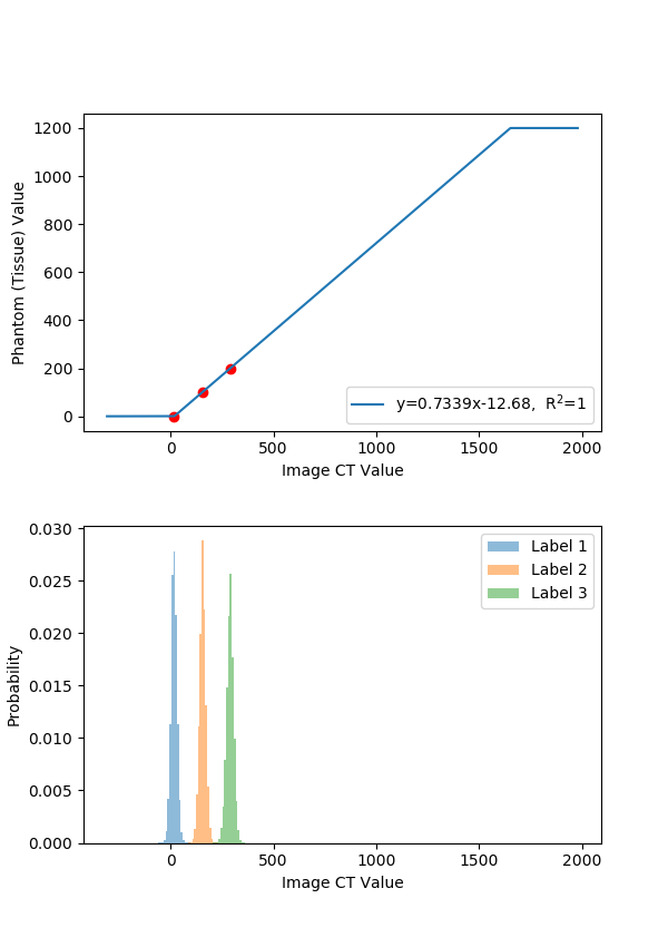
This scripts computes tissue density values (e.g. BMD) from CT values (Hounsfield units, HUs). Such CT value modification is known as calibration and gives quantitative CT numbers for a considered tissue density e.g. bone.
A gray-level file (HUs) and a corresponding mask which gives image regions with known tissue densities (the phantom chambers) have to be provided in order to establish the calibration law. These calibration parameters are use to calibrate a given image.
Either the gray-level HU input file including the phantom is calibrated or an other given gray-level file can be calibrated. Polynomial fitting including cut-offs by given limits (e.g. BMD values) is possible.
Several output options are available like image files, mid-planes, or text output files (csv format).
Usage
Module:
import ctcal
Command line:
python ctcal.py ...

   -inp   testPhCT.mhd
   -inl   testLabel.mhd
   -tiss  1;;0;;;2;;100;;;3;;200
  [-show  OFF                   ]
  [-inc   testCalib.mhd         ]
  [-form] format                ]
  [-out   testOut.mhd           ]
  [-mid   test.png              ]
  [-deg   1                     ]
  [-limit 0;1400                ]
  [-txt   testOut.txt           ]
  [-mod   w                     ]
  [-shist OFF
  [-gui                         ]
  [-doc                         ]
  [-help                        ]
Parameters
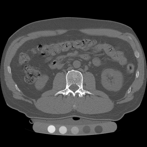
- -inp
: str
CT (Phantom) Input File. A gray-level HUs file which contains the phantom. This file is used to average the gray-values within the phantom chambers (regions with known tissue density). The labelled mask for these chambers is provided by the ‘inl’ option. Possible extensions are:
‘.mhd’ : MetaImage file(ITK). Consist of a meta data file ‘.mhd’ and a binary ‘.raw’ file. The mhd file contains all important informations. It is readable by a text editor. The data itself are stored in a separate raw file. This or the ‘.nhdr’ is the recommended file format.
‘.nhdr’ : NRRD image file composed of a header ‘.nhdr’ and a binary ‘.raw’ file like the mhd format. This is the recommended file format if transformations are important and Slicer3D is used.
‘.isq’ : SCANCO ‘isq’ file format (primary format of SCANCO scanners)
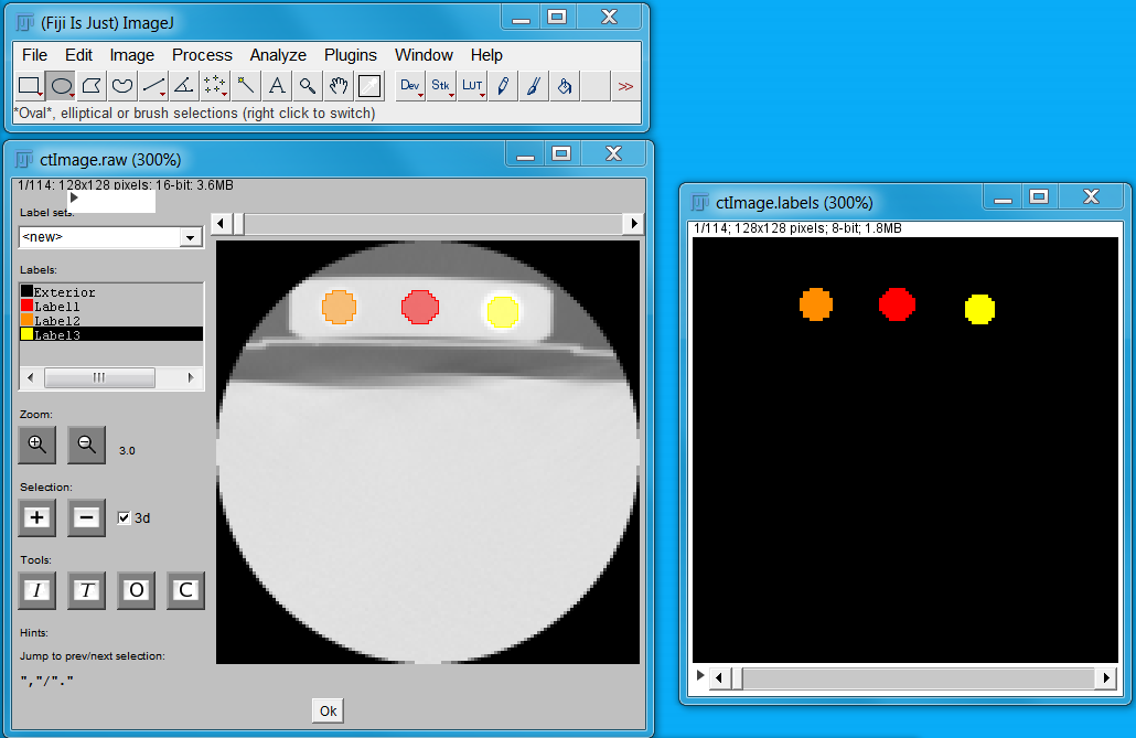
- -inl
: str
Label Input File. The image provides the masked phantom chambers with known tissue density. These regions have values greater than 0. Each phantom chamber has to have an unique label e.g. 1,2,3,etc. The file shape has to fit to the file given in ‘inp’ option. These labels could be done interactively using the Viewer in medtool or, e.g., the segmentation editor of Fiji.
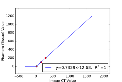
- -tiss
: Label;Density (str)
Tissue Densities or Phantom Values. This list contains the labels from the file given in the ‘inl’ option and the know tissue density (e.g. mgHA/ccm). These are the known ‘y’ value of the calibration law
Tissue
Density
  |         x
  |     x
  |  x
  |____________ CT Image
                Values
The x-axis is represented by the ‘CT Image Values’ which are the averages computed from the file given in the ‘inp’ option.
Optional Parameters
- -show
: flag (str)
Show Regression. If this option is active the plot of the calibration including the limits are shown.
- -inc
: str
CT Input File. If this file is given it will be used for calibration instead of the file given in the ‘inp’ option.
- -out
: str
Calibrated CT Output File. This file contains the quantitative information e.g. mgHA/ccm as quantities.
- -form
: format
Byte format of image file (voxel data) for RAW. Currently implemented B…uint8, H…unit16, h…int16, i…int32, f…float32 Note that the supported format depend on the platform 32 or 64 bit. Depending on the format the file has to be converted to with ‘scale’ option first e.g. for uint8 gray-values from 0-255 are required.
- -mid
: str
Output mid-planes computed from the calibrated CT output file.
- -fct
: value (str)
Fitted calibration function. ‘poly’ or ‘exp’ are implemented. If ‘exp’ is selected then the option ‘deg’ will be ignored. Default = ‘poly’.
- -deg
: value (int)
Poly Fit Degree. The degree of the fit. For example ‘deg=1’ for a linear of ‘deg=2’ for a quadratic fit. Only used if ‘fct’=’poly’, otherwise the option is skipped. Default=1.
- -limit
: Min;Max (list[float])
Min/Max Density. The minimum and maximum allowed tissue densities that are used during calibration. For example, in case of bone this could be ‘0’-‘1200’.
- -txt
: str
Text Output File. Writes the computed calibration information to a CSV file which can be viewed with a spreadsheet editor.
- -mod
: str
Write mode for writing the ‘txt’ file (python style). It can be:
‘w’ (create new file) write header + data) and
‘a’ (append to file, write data).
- -shist
: flag (str)
Shows the histograms gray-vaules of the masked phantom areas.
- -gui
:
Print gui string on stdout.
- -doc
:
Print default doc string (__doc__) on stdout..
- -help
:
Print help string (extended __doc__) on stdout..
Info
File: ctcal.py
Author: D. H. Pahr
Converter FEA - Abaqus, CalculiX
This script generates a finite element model from a 3D image as well as numerous other parameters. The gray vaules can be used as variables for the generation of density dependent material cards. Note sets can be automatically created on the 3D image boundary to easily apply boundary conditions. A template file is created in the background and medtools Image-Processor script is used to create the FEA input deck.
The script should help to quickly create an FE input deck from a template file. However, some basic knowledge of the FE method is required. This input file can be analyzed with the free software package Calculix (see http://www.calculix.de/).
Usage
Module:
import imgToFe
Command line:
python imgToFe.py ...

   -in       image.mhd
   -out      model.inp
  [-smooth   5;0.6307;0.1;0;1;0.05                 ]
  [-matpow   1-250;20000;0.3;2;...                 ]
  [-matelas  251;1000;0.3;...                      ]
  [-nsetfa   flag                                  ]
  [-disp     ALL_NODE_B;1-3;0.0;ALL_NODE_T;3;0.1   ]
  [-force    ALL_NODE_N;3;100.                     ]
  [-step     Static                                ]
  [-spar     0.2;1.0                               ]
  [-nodefrd  U;RF                                  ]
  [-elemfrd  S;E;ENER                              ]
  [-nodedat  ALL_NODE_T;RF                         ]
  [-gui                                            ]
  [-doc                                            ]
  [-help                                           ]
Parameters
- -in
: filename (str)
Image file name. This image is converted into a finite element model. It usually contains gray values from 0 to 255. Note:
GV=0 are per default pores, i.e. no elements are created
GV=1..250 are used for bone tissue (density dependent)
GV=251..255 are used for other elstic materials (polymer, metal , …)
Supported file formats are:
‘.mhd’ : MetaImage file(ITK). Consist of a meta data file ‘.mhd’ and a binary ‘.raw’ file. The mhd file contains all important informations. It is readable by a text editor. The data itself are stored in a separate raw file.
‘.nhdr’ : NRRD image file composed of a header ‘.nhdr’ and a binary ‘.raw’ file like the mhd format.
- -out
: filename (str)
FEA job file name. This is the created FEA input deck which can be analyzed with the free software package Calculix. The output format is very similar to Abaqus’s ‘.inp’ file.
For the creation of this file, a template file is created For example, if a the filename is ‘test.inp’, the template file is called ‘test_temp.inp’. This template file could be modified and used in medtool’s Image-Processor to create an input deck with more flexibility.
Optional Parameters
- -smooth
: niter;lambda;kPB;interface;boundary;jacobian (list[str])
Mesh smoothing. This option is smoothing the voxel type mesh before creating the output.
‘niter’ is the number of iterations. One iteration means forward (with lambda) and backward smoothing (with mu) smoothing.
‘lambda’ scaling factor (0<lambda<1)
‘kPB’ pass-band frequency kPB (note kPB=1/lambda+1/mu > 0) => mu
‘interface’ on/off switch for including near interface node smoothing. This option is in the current Fortran code not implemented!!
‘boundary’ boundary smoothing id, have to be provided with
boundary=0 … no smoothing of boundary elements/nodes
boundary=1 … smoothing of boundary elements/nodes but preserving cutting planes
boundary=2 … smoothing of boundary elements/nodes
‘jacobian’ minimal allowed scaled Jacobian. E.g. 0.02 means the smallest allowed volume change is 2% of the initial volume.
- -matelas
: GV;E;nu;… (list[str])
Elastic material card for isotropic material e.g. a polymer. The gray value ‘GV’ can be a single value e.g. ‘251’ or a range e.g. ‘251-254’. It is converted to a linear elastic material with Young’s module ‘E’ and Poisson ratio ‘nu’.
Note: that gray values given here and in the ‘matpow’ or option have to be unique e.g. must not overlap.
Repeat this line if needed.
- -matpow
: GV;E0;nu;k (list[str])
Elastic material card for a gray-level dependent material using a power law e.g. for bone. The variable ‘GV’ gives the gray value range e.g. ‘1-250’. The power law for the mapping is given by the formula
E = E0 * (GV/nGV)**k
with :
‘E0’ .. tissue modulus in MPa
‘nu’ .. Poisson number e.g. 0.3-0.4
‘k’ .. power constant.
‘GV’ .. gray value of current voxel e.g. between 1-250
‘nGV’ .. number of gray values e.g 250 in this example
‘GV/nGV’ .. density between 0 and 1.
Note: The ‘grayvalue’ given here and in the ‘matelas’ option have to be unique e.g. must not overlap.
- -nsetfa
: flag (str)
Create node set of boundig box faces. The faces bounding box of the image are denoted as
                            ALL_NODE_N

                   o------------------o
                  /|                 /|
                 /                  / |
                /  |  ALL_NODE_T   /  |
               /                  /   |
              /    |             /    |
             o------------------o   <<<<< ALL_NODE_E
             |     |            |     |
ALL_NODE_W >>|>>   o- - - - - - | - - o
             |    /             |    /
             |                  |   /
             |  /   ALL_NODE_B  |  /
             |                  | /
             |/                 |/
             o------------------o

              ALL_NODE_S
If flag is ‘ON’ the following node sets are generated: ALL_NODE_S, ALL_NODE_N, ALL_NODE_E, ALL_NODE_W, ALL_NODE_T, ALL_NODE_B. These sets can be used to apply displacements in ‘disp’ or forces in ‘forc’ option as well as for result output.
- -disp
: region;dofs;mag;… (list[str])
Displacement boundary condition. The variables have the following meaning :
‘region’ .. node number or node set label. If ‘nsetfa’ is active e.g. ALL_NODE_B.
‘dofs’ .. degree of freedom constrained. A range (first and last dof constrained) e.g. 1-3 or single value can be given (1,2, or 3).
‘mag’ .. magnitude of the prescribed displacement.
Repeat this line if needed.
- -force
: region;dof;mag;… (list[st])
Force boundary condition. The variables have the following meaning :
‘region’ .. node number or node set label. If ‘nsetfa’ is active e.g. ALL_NODE_B.
‘dofs’ .. degree of freedom. A single value can be given (1,2, or 3).
‘mag’ .. magnitude of the prescribed nodal force.
Repeat this line if needed.
- -step
: type (str)
Analysis step type. This option is used to select a linear static analysis step (‘STATIC’ - Default) or non-linear static analysis step (‘STATIC_NLGEOM’). In case of ‘STATIC_NLGEOM’, analysis parameters can be given with ‘spar’ option.
- -spar
: increment;time_period (list[float])
Analysis parameters for a non-linear static analysis step. These parameters are omitted in case of a ‘STATIC’ analysis. The inputs are :
Time increment (default 1.).
Time period of the step (default 1.).
- -nodefrd
: var1;var2;var3;var4 (list[str])
Node results FRD. Write selected nodal variables in file jobname.frd. The following variables can be selected:
RF .. External forces
U .. Displacements
- -elemfrd
: var1;var2;var3;var4 (list[str])
Element results FRD. Write selected element variables in file jobname.frd. The following variables can be selected:
E .. total Lagrangian strain for (hyper)elastic materials and incremental plasticity
ENER .. the energy density.
S .. true (Cauchy) stress in structures.
- -nodedat
: region;var1;var2;var3 (list[str])
Node results DAT. This option is used to print selected nodal variables in file jobname.dat. The following variables can be selected:
RF .. External forces
U .. Displacements
- -gui
:
Print gui string on stdout.
- -doc
:
Print default doc string (__doc__) on stdout..
- -help
:
Print help string (extended __doc__) on stdout..
Info
File: imgToFe.py
Author: D. H. Pahr
Converter - Mhd to uFE
Script reads a binary voxel file using ‘mhd’ format together with an
FE Template File (same as for mic but with *USER PARAMETER) and writes
the HDF5 file for ParFE, ParOSol, ParFeap, Ansys
Usage
Command line:
pfeToH5  ...

  -in       InputFileName
  -temp     TemplateFileName
  -out      OutputFileName
  [-type]   FileType            [optional]
Parameters
- -in
: Name of the voxel model input file. In the current version it has to be segmented. Only the voxel with a gray vale given in
*USER DIRECT PROPERTYare to be converted to hexahedral elements.- -temp
: Name of an ParFe Template file. Supported commands:
*USER HEADER
*USER DIRECT PROPERTY
*USER PARAMETER
*USER NODE
*USER ELEMENT
*USER BC1
*USER BC2
*USER BC3
Example:
########################################################################
## ParFe example template input file
## NOTE: voxel size has is given in mm, E-Modulus in MPa
########################################################################
## Control parameters, inserted by the script
*USER HEADER
########################################################################
## First line  : nMatParameter (E,nu), nMatTypes (gray values)
## Second line : matId_1, E_1, nu_1
## Third line  : matId_2, E_2, nu_2
*USER DIRECT PROPERTY
2 2
75 20000. 0.3
255 3000. 0.3
########################################################################
## First line : conversion_tol, iter_limit
*USER PARAMETER
0.000010 10000
########################################################################
## Nodal coordinates, inserted by the script
*USER NODE
########################################################################
## Element connectivity, inserted by the script
*USER ELEMENT
########################################################################
## BC1 Fixed DISPLACEMENT
## First line  :  number of BC sets
## Second line :  SetName, x, y, z (0->constrained, 1->free)
##                The free BC may set with BC2 or BC3 below.
## NOTE: Edge nodes not checked. They may appear twice !!!
*USER BC1
2
ALL_NODE_B 0 0 0
ALL_NODE_T 0 0 1
########################################################################
## BC2: Load at nodes
## 1st: Command - *USER BC2
## 2nd: number of given lines specifing the BCs
## 3rd: 'nset name', xLoad, yLoad, zLoad    (loads are real numbers [N])
## TYPE 1 : DIRECT, 'nset name', Fx(N), Fy(N), Fz(N)
##          Example : DIRECT ALL_NODE_T 1.5 1.3 2.8  or
##                    ID_NODE_6000 0.0 0.0 1.0
## TYPE 2 : CONSISTENT, 'nset name', Fx(N), Fy(N), Fz(N)
##          Example : CONSISTENT ALL_NODE_T 1.5 1.3 2.8
## NOTE: Edge nodes not checked !!! They may appear twice with
##       different BCs!
##       Clean model before running analysis!
*USER BC2
0
########################################################################
## BC3 applied DISPLACEMENT
## First line  :  number of BC sets
## Second line :  SetName, x, y, z (displacement in mm)
## NOTE: Edge nodes not checked. They may appear twice !!!
########################################################################
## BC3 Prescribed (non-zero) displacement at nodes
## 1st: Command - *USER BC3
## 2nd: Number of given lines specifing the BCs
## 3rd: Data for BCs which can be '([]...means optional)
## TYPE 1 : [DIRECT], 'nset name', 'coord dir (1,2,3)', 'disp (mm)'
##          Example : [DIRECT] ALL_NODE_T 3 -0.1 (or ALL_NODE_T 3 -0.1)
##
## TYPE 2 : KIN_COUPLING , 'couple_dir (1,2,3,12,13,23,123)' ...
##          pO01, pO02, pO03, pOA1, pOA2, pOA3, pOA1, pOA2, pOA3, ...
##          pN01, pN02, pN03, pNA1, pNA2, pNA3, pNA1, pNA2, pNA3, ...
##          l_ref, 'l_dir (1,2,3,12,13,23,123)' (l_ref=0.0 .. no scale)
##          Example : KIN_COUPLING ALL_NODE_T 123 ...
##                    1  0.0 0.0 0.0  1.0 0.0 0.0  0.0 1.0 0.0 ...
##                    1  0.1 0.0 0.0  1.0 0.0 0.0  0.0 1.0 0.0 ...
##                    0.3 123                           (or simply: 0.0)
##          Explanations :
##            KIN_COUPLING : predefined keyword to indicate this BC type.
##                           The coupling is realized by a transformation
##                           from an old to a new basis
##            coupling_dir : A number out of 1,2,3,12,13,23,123
##                           1 means coupling in 1 direction, 12 means
##                           couling of dofs in 1 and 2 direction, etc
##            pO01, ... : points ('p') given the old ('O') basis point
##                        zero ('0') in the first ('1') direction
##                        In total three points 0,A,B need to be given
##                        (see figure below). These are positions not
##                        normal vectors and need not to be perpendicular
##                        The old basis is computed from these points
##                        where 0 is the base point.
##            pN01, ... : similar as pO01, ... These points are needed to
##                        compute the new basis (see figure).
##            l_ref     : a reference length e.g. length of a unit cell.
##                        Switched of if value is 0.0. In this case
##                        l_dir needs not to be given and a rigid
##                        transformation is done.  For more details
##                        see below.
##            l_dir     : Considered 1,2,3 components to compute the
##                        distance vector. For more details see below.
##
##            Based on these inputs the displacment of a node pUX is
##            computed from (non-rigid transformation):
##
##                            vUX   = ( pNX - pOX ) * scale
##                            scale = lX / l_ref
##                            lX    = | pOX - pO0 |
##
##            vUX        : displacement vector of a point X.
##            lX         : distance between point '0' and point 'X' both
##                         given in the old ('O') system. l_dir specifies
##                         which components of this vector are considered
##                         in the computation of this norm.
##            scale      : Scaling of the movement of a point X. This is
##                         based on lX and the given l_ref. E.g. in case
##                         of KUBCs this allows to give uniformly
##                         increasing displacements.
##
## NOTE:
##    - Double BCs are checked! First given BCs will be taken.
##    - You can use '...' and continue entry in next line
##    - nset name ID_NODE is currently not implemented
##
*USER BC3
1
KIN_COUPLING ALL_NODE_T 3 ...
0 0 3    1 0 3    0 1 3 ...
0 0 3.1  1 0 3.1  0 1 3.1 ...
0.1 12
#ALL_NODE_T 3 -0.1
########################################################################
## Top node set:  #nodes; nd#
0
## Btm node set:  #nodes; nd#
0
## Top elmt set:  #els;   el#
0
## Btm elmt set:  #els;   el#
0
########################################################################
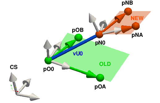
- -out
: Name of the hdf5 parfe data file which should be written.
- -type
: Output file type ‘parfe’, ‘ansys’, ‘feap’, ‘parosol’
- -gui
: Print GUI string on stdout
- -help
: Print usage
Info
File: pfeToH5.cpp
Author: D. H. Pahr, Elankumaran
Script Medtool - 3D Slicer Bridge
This script starts 3D Slicer and loads a background image. It is possible to switch between a reduced and full Slicer 3D view. After clicking the “Back to medtool” button in the 3D Slicer, data are saved, and the app is closed. After the return, medtool continues to execute the next script.
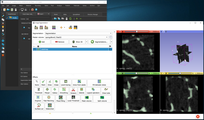
The following apps are implemented:
view
roi
segmentation
The ‘view’ app allows to load optionally a foreground image as well as label map image into 3D Slicer. The image can then be viewed interactively in Slicer 3D.
The ‘roi’ app loads a background and a cubical ROI. The ROI can then be manipulated interactively in Slicer 3D. After returning to medtool, the bounding box is written in a text file which can be read with medtool’s image processor (‘roitxt’ option).
The ‘segmentation’ app loads a background as well as optionally a label image into 3D Slicer, and starts the segmentation editor. The image can then be segmented interactively in Slicer 3D. After returning to medtool, the new label map is saved.
Sketch of the communication wiht 3D Slicer:
     medtool
 _______________           extension               reduced              full
|               |           module                3D Slicer           3D Slicer
| script        |       _________________       ________________       _______
| script        |      |                 |     |                |     |       |
| slicer bridge | -->  | reduced GUI     | --> | open Slicer    | --> |       |
| script        | <--  | back to medtool | <-- | back to module | <-- |       |
|_______________|      |___|_____________|     |________________|     |_______|
                           |
                           ---> save data
The extensions are tested on 3D Slicer Version 4.11. Installation procedure:
install 3D Slicer. 3D Slicer is not part of medtool and needs to be installed separately for your OS
open 3D Slicer
install the ‘SegmentationEditorExtraEffects’ extension from ‘View’ - ‘Extension Manager’ menu
link all extension modules (delivered with medtool in ‘Slicer’ folder) in 3D Slicer under ‘Edit’ - ‘Application Settings’ - ‘Modules’ - ‘Additional module paths’. It needs to be done for all extensions individually.
close 3D Slicer
set the Slicer executable in medtool via ‘Run Settings’ - ‘3D Slicer Executeable’
create a slicer bridge script in medtool via ‘Image’ - ‘3D Slicer’
run the slicer bridge script
Usage
Module:
import medtoolSlicerBridge
Command line:
python edtoolSlicerBridge.py ...

   -bgv  background.mhd
   -app  selectedApp
  [-lmv  labelmap.mhd        ]
  [-fgv  foreground.mhd      ]
  [-opa  0.5                 ]
  [-roi  roi.txt             ]
  [-osg  outsegmentation.mhd ]
  [-isg  insegmentation.mhd  ]
  [-orm  axes                ]
  [-rul  yes                 ]
  [-gui                      ]
  [-doc                      ]
  [-help                     ]
Parameters
- -bgv
: filename (str)
Background volume.
- -app
: combo (view;roi;segmentation)
App selection. Impemented are ‘view’, ‘roi’, and ‘segmentation’.
Optional Parameters
- -lmv
: filename (str)
Label map volume for ‘view’ app.
- -fgv
: filename (str)
Foreground volume for ‘view’ app.
- -opa
: number (*)
Opacity of the forground volume for ‘view’ app.
- -roi
: filename (str)
ROI bounding box file for ‘roi’ app.
- -osg
: filename (str)
Output Segmentation volume for ‘segmentation’ app.
- -isg
: filename (str)
Input segmentation for ‘segmentation’ app.
- -orm
: combo (cube;human;axes)
Orientation Marker for all apps.
- -rul
: flag (*)
Show Ruler for all apps.
- -gui
:
Print gui string on stdout.
- -doc
:
Print default doc string (__doc__) on stdout..
- -help
:
Print help string (extended __doc__) on stdout..
Info
File: medtool_slicer.py
Author: D. H. Pahr
Script 3D Viewer
This script allows the call of external image viewers via SimpleITK. (see https://simpleitk.readthedocs.io/en/latest/link_ImageViewing_docs.html)
By default Fiji/ImageJ is called if it is installed under:
On Windows: in your user directory (e.g. C:Usersyour_user_nameFiji.app). On Linux: in ~/bin .
Other image viewer application (e.g. ITK-SNAP, 3D Slicer) can be chosen with or without additional command line arguments.
Fiji Screenshot:
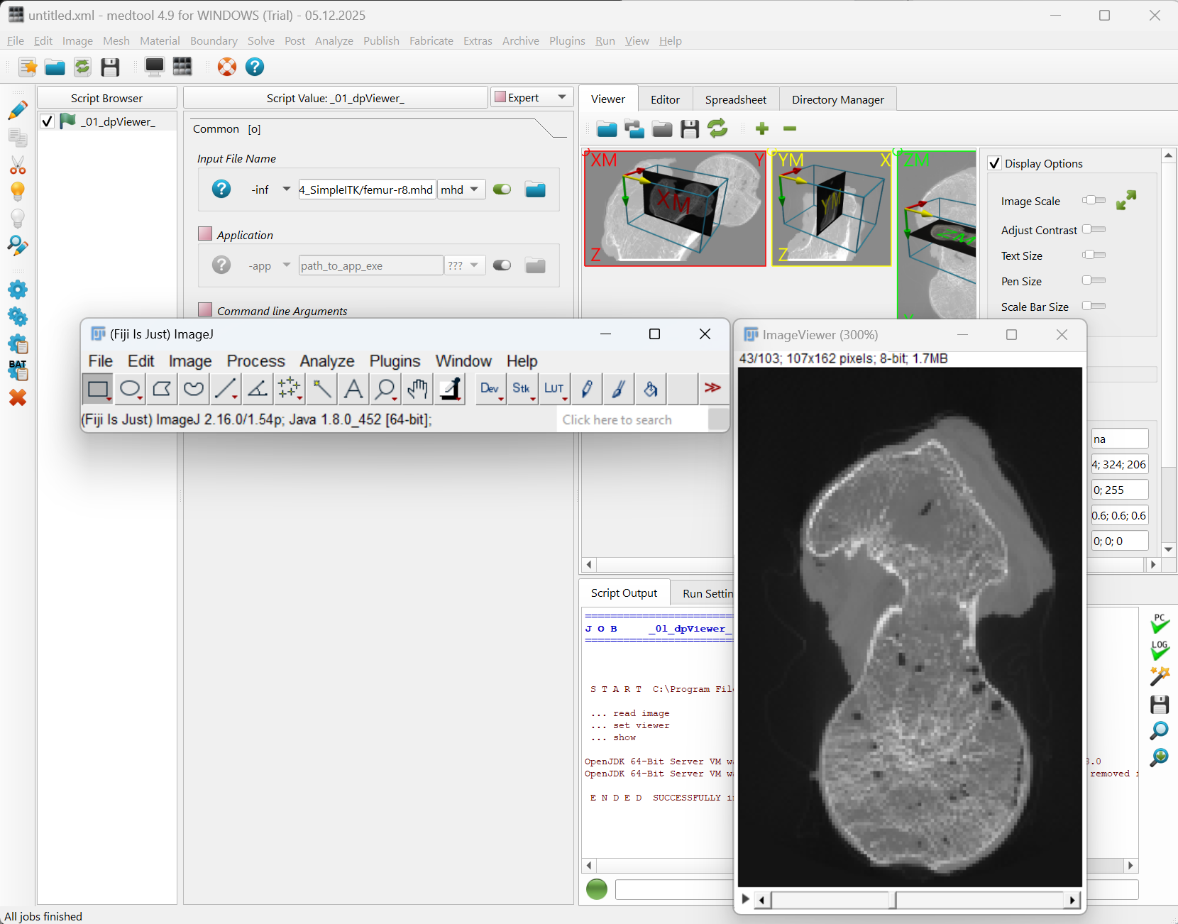
ITK-Snap Screenshot:
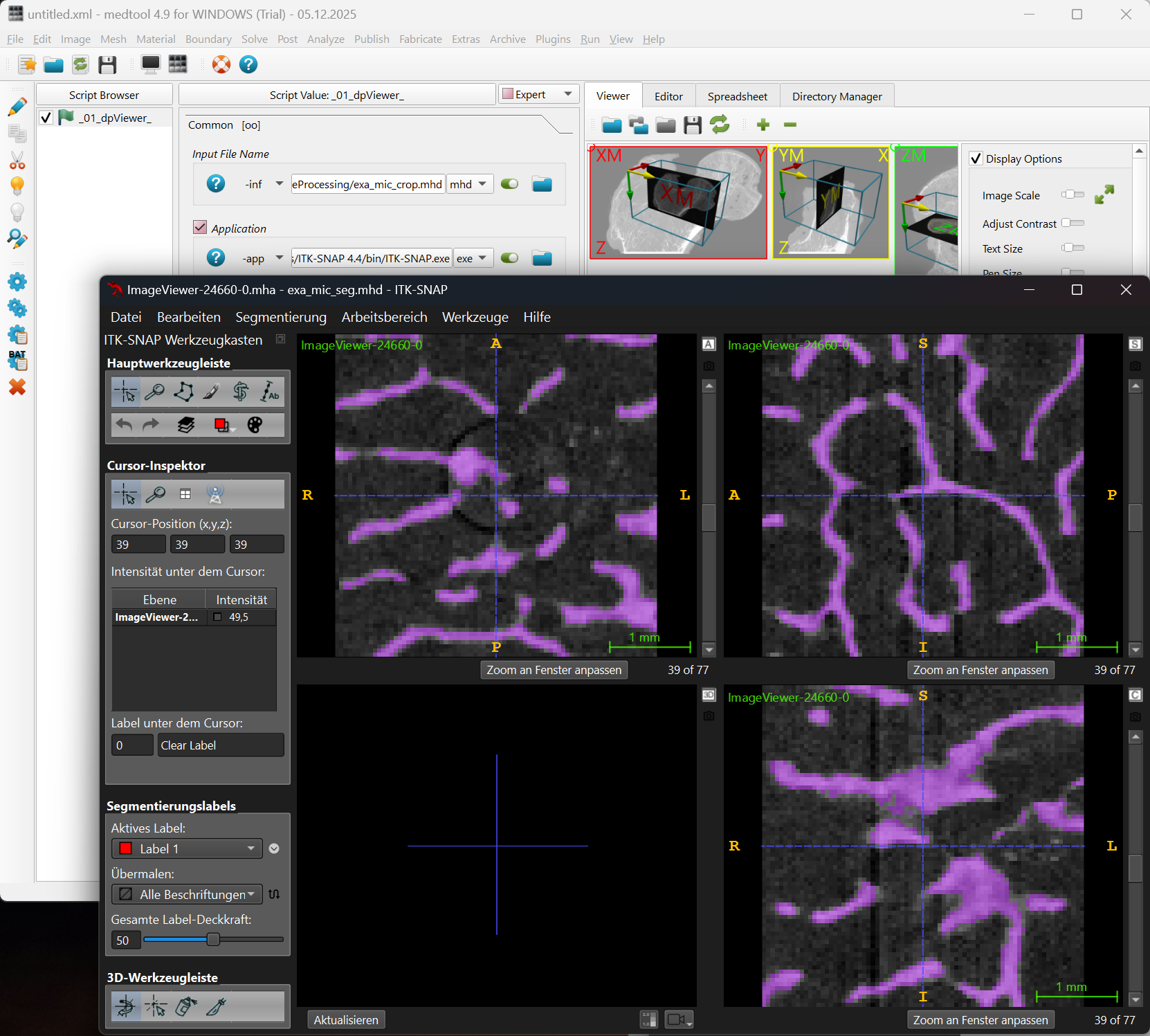
3D Slicer Screenshot with second loaded image:
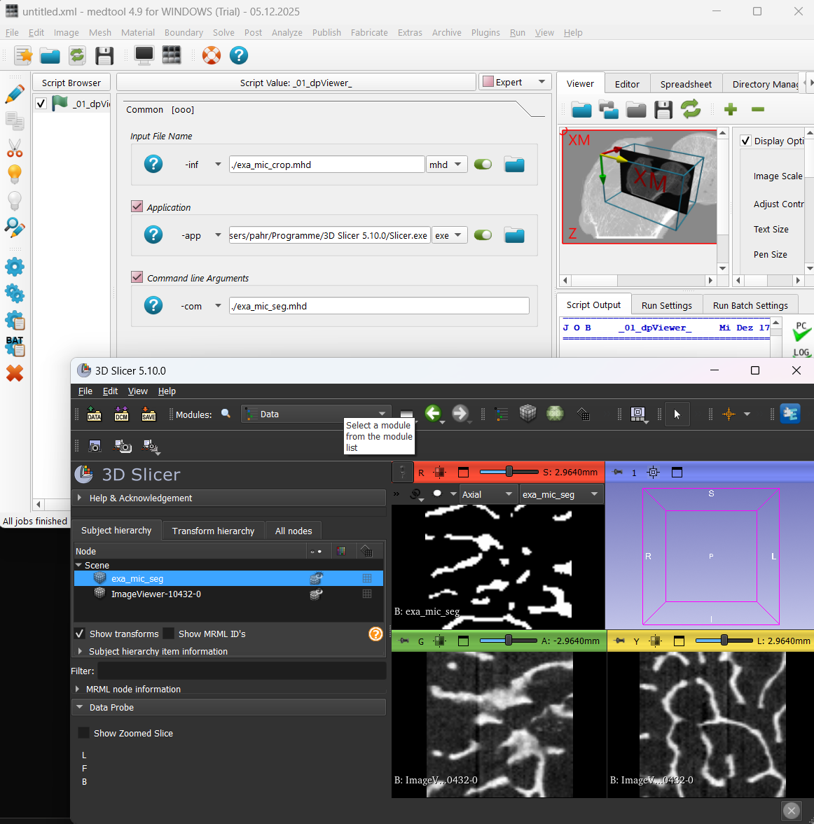
Usage
Module:
import dpViewer
Command line:
python dpViewer.py ...

   -inf     testIn.mhd
  [-app     path_to_app_exe]
  [-com     -z;2           ]
  [-gui                    ]
  [-doc                    ]
  [-help                   ]
  [-version                ]
  [-author                 ]
Parameters
- -inf
: filename (str)
Image input file name.
Optional Parameters
- -app
: filename (str)
Viewer application executeable file name.
- -com
: number (list[str])
Additional command line arguments of the viewer application.
- -gui
:
Print gui string on stdout.
- -doc
:
Print default doc string (__doc__) on stdout.
- -help
:
Print help string (extended __doc__) on stdout.
- -version
:
Print the version on stdout.
- -author
:
Print the author on stdout.
Info
File: dpViewer.py
Author: D. H. Pahr
Mesh
The meshing module contains interfaces to freely available meshing software as well as specialized meshing algorithm. They are designed to create high-quality meshes which are usually used for simulation models. A unstructured (finite element) mesh converter allows to convert between different file formats.
2D - Isosurfer
Script is an interface to isosurf see: http://mi.eng.cam.ac.uk/~gmt11/software/isosurf/isosurf.html
Isosurf is not part of medtool. Executables from external resources are added for different platforms without any warranty. Isosurf might need to be compiled / installed by the user.
EXAMPLE:
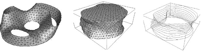
The input data is first read, then thresholded at a user-defined value, resulting in a set of binary cross-sections. These cross-sections can optionally be filtered using a morphological opening and/or closing with a disc size appropriate to the sampling resolution. This operation ensures that the contours do not contain features which are smaller than the sampling resolution. If no morphological filtering is used, the original data values are used to define the location of the cross section in each slice more accurately - this can result in smoother surfaces at very high resolution.
Having done this, each cross section is transformed such that pixels in the image represent the minimum distance to the contour in that image (discussed further in a technical report). This improves both the interpolation of the surface and the smoothness of the surface display.
Surface triangulation is performed at a user defined resolution, using regularized marching tetrahedra (described in a technical report). If this resolution is greater than the inter-plane spacing (the z resolution), then additional planes are interpolated using disc-guided interpolation (described in another technical report). For faster though less realistic results, shape-based interpolation can optionally be used instead of the previous technique. Obviously higher resolutions will lead to greater surface detail, but also greater numbers of triangles - and therefore longer processing times for visualization.
The filtered cross sections are also extracted and saved to a file as vectors which can be displayed in 3-D - this can be helpful in defining a sensible threshold for the input data.
As an extremely rough guide, triangles can be generated at about 4000 per second on typical modern hardware - plus several seconds for pre-processing (more if a very large filter is required due to a very low sampling resolution). This drops to 1000 or less triangles per second if the cross-sections also require interpolation - in this case the processing time is dependent on the complexity of the input data.
Usage
Command line:
python isosurfRun.py  ...

  -exe filename
  -i   filename
  -o   filename
  -d   nVox1;nVox2;nVox3
  -f   binFormat          (optional)
  -s   len1;len2;len3     (optional)
  -t   lowThres;highThres (optional)
  -r   factor             (optional)
  -m   type               (optional)
  -c                      (optional)
  -v                      (optional)
  -a                      (optional)
  -q                      (optional)
  -h                      (optional)
Parameters
-exe : filename
The used isosurf executable. You find one executable in the medtool install directory (->MEDTOOLPATH) which is used as default
- -i
: filename
Input file name. ‘filename’ is the full name of the file containing the input data. Default is ‘data.bin’.
- -o
: filename
Output file name is the full name of the file containing surface information. This option is not available in isosurf. It simply moves the surface.off file to this file name. The contour file will be still ‘countours.off’.
- -d
: nVox1;nVox2;nVox3
Data dimensions in 1, 2 and 3 are the dimensions of the input data array. These are integers.
- -f
: binFormat
The binary storage data format of the input data. ‘format’ can be ‘c’ for unsigned char, ‘u’ for unsigned short or ‘s’ for short. The default is unsigned char.
- -s
: len1;len2;len3
Data scale factors. The actual physical distance represented by one step in each of the 1, 2 and 3 directions. These are floats. The default is 1.0 in all directions.
- -t
: lowThres;highThres
Iso-surface threshold. The object is extracted for which the data is greater than or equal to ‘lowThres’, and less than or equal to ‘highThres’, both of which are integers. The default values are 1,255.
- -r
: factor
‘factor’ defines the resolution of the grid which is used to sample the data and from which the iso-surface is extracted. This is a float, in scaled units, as per the given data scale factors. Default value is 1.0.
- -m
: type
The type of filtering operation performed on the thresholded cross- sections. ‘type’ can be ‘o’ for opening, ‘c’ for closing, ‘b’ for both or ‘n’ for neither. The default is both, which is appropriate for data containing small objects and holes. If neither is used, the data will not be filtered, but the grey scale values will be used to locate the cross-section more accurately within each slice.
- -c
: None
Exclude end caps. Causes the first and last planes not to be triangulated.
- -v
: None
Generate VRML rather than OOGL output.
- -a
: None
Centralize the output data. Causes the output mesh to be centered around the point (0, 0, 0). The scale remains unaltered.
- -q
: None
Quick interpolation. If the data requires interpolation, this causes shape-based interpolation to be used, rather than the default maximal disc guided interpolation.
- -h
: Help. Displays a brief help screen.
Info
File: isosurfRun.py
Author: D. H. Pahr
2D - VXI Mesher
The mesher extracts interfaces between compartments given via segmented voxel images. This voxel-based interfaces (zig-zag surfaces) are extracted and are smoothed afterwards. Different iso-surfaces extraction algorithm are implemented.
The initial voxel model can be re-coarsened by a factor in order to obtain coarser meshes.
The interface surfaces can be written to output files. Depending on the file format, interface ids are used as element set definitions.
Usage
Module:
import dpMesher
Command line:
python dpMesher.py ...

   -in     image.mhd
  [-out    testIso.case ]
  [-resf   2            ]
  [-stype  "vxi_m"      ]
  [-offset "ON"         ]
  [-bfeat  "ON"         ]
  [-smooth 10:0.6307:0.1]
  [-gui                 ]
  [-doc                 ]
  [-help                ]
Parameters
- -in
: filename
Name of the voxel file which should be converted. The file type is recognized by the file extension. The
micmodule (image processor) is used to read the images and all implemented file formats ofmiccan be used. Voxel data has to be UINT8 (0..255). Interfaces are generated between two voxel with different grayvalues.
Optional Parameters
- -out
: filename
Name of the surface output file. File formats are :
‘.case’: PARAVIEW : Ensight gold format (same as ‘.geo’)
‘.inp’: ABAQUS input file
‘.off’: Geomview file
‘.msh’: GMSH file
‘.stl’: stereolithography file
‘.surf’: netgen’s surface mesh file
‘.smesh’: tetgen’s surface mesh file
‘.vtk’: vtk ASCII file
- -resf
: int
Resampling data by factor. The images can be resampled (re-coarsened) by a factor before the analysis. The thresholding is simply done by found the new image gray-value. Therefore, the grayvalues of segmented images should be like 1,2,3,4 and not 10, 20, 30 because in the latter case new gray values are generated.
Note that the change of the image resolution may influence the outcome considerably and should be avoided.
- -stype
: str
Surface mehser type. Implemented types are :
‘vxi_m’: voxel interface extraction followed by a smoothing based on local node moving
‘vxi_mi’: voxel interface extraction followed by a smoothing based on local node moving with one iteration
‘vxi_tb’: voxel interface extraction followed by a smoothing based on a taubin smoothing
The default value is ‘vxi_m’.
- -offset
: str If this flag is switched on (value ‘ON’), the offset from the image will be taken into account. Otherwise the offset is 0,0,0.
The default value is ‘offset’=’ON’
- -bfeat
: str
If this flag is switched on (value ‘ON’), the boundary feature is preserved. Otherwise (‘OFF’) the boundary nodes are treated as internal nodes and smoothed.
-smooth : list
Smooth surface mesh. This filter becomes active if ‘stype’ is ‘vxi_tb’. The implementation follows Taubin’s smoothing algorithm (see, Taubin, Eurographics 2000, Boyd and Mueller 2006). PARAM: niter;lambda;kPB;jacobian;areaChange
‘niter’ number of iterations. One iteration means forward (with lambda) and backward smoothing (with mu) smoothing i.e. 2 smoothing steps.
‘lambda’ scaling factor (0<lambda<1)
‘kPB’ pass-band frequency kPB (note kPB=1/lambda+1/mu > 0) => mu
‘jacobian’ minimal allowed scaled Jacobian. E.g. 0.02 means the smallest allowed volume change is 2% of the initial volume.
‘areaChange’ maximal allowed change of triangle area during smoothing. E.g. 0.4 means that the current triangle area is allowed to be 40% bigger or smaller than the initial triangle area.
- -out
: str Output file name. This is the name of an output file name which includes the interface surfaces. The mesh can be displayed e.g. with Paraview or similar.
- -bin
: flag
Toggles writing binary STL files ‘ON’ or ‘OFF’.
- -gui
: Print gui string on stdout.
- -doc
: Print default doc string (__doc__) on stdout..
- -help
: Print help string (extended __doc__) on stdout..
Info
File: dpMesher.py
Author: D. H. Pahr
3D - CGAL Mesher
This CGAL mesher is devoted to the direct generation of isotropic 2D and 3D meshes of gray-level domains. This domain is a region of 3D space, bounded, and characterize by a specific gray-level. The mesher generates tetrahedral meshed (3d) for every gray-level. Between the gray-level triangulated meshes (2d) can be written out.
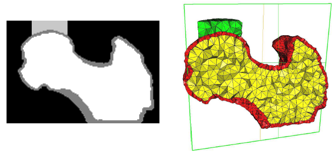
Abaqus, medit or tetgen output is possible. Files can be converted to other formts using the medtool converter.
The mesher is a fast and robust way to generated 2D and 3D meshes of gray-level domains. It is based on CGAL - 3D Mesh Generation - mesh_3D_image.cpp
Input images are labelled gray-value images. Voxel data types have to be UINT8 (0..255). Inria ‘inr.gz’ or VTK/ITK ‘mhd’ file formats are implemented!
Usage
Command line:
cgalSurfMesher ...

  -in       filename
  -out      filename
  -osp      output_specifier
  -csize    cell_size
  -fdist    facet_distance
  -fsize    facet_size
  -fangle   facet_angle
  -cratio   cell_radius_edge_ratio
  -rsize    cell_size
  -riter    iteration_number
  -opt      optimizerList
  -time     optimizerLimitTime
Parameters
- -in
: filename
Name of the voxel file which should be converted. Currently ‘inr.gz’ (Inria Image Files) or VTK/ITK’s mhd format is implement.
- -out
: filename
Name of the surface output files. File formats are :
mesh: medit ‘mesh’ file
inp: Abaqus input file format
am: AVIZO mesh format
tg: tetgen file format
In case of tetgen the dummy file extension ‘tg’ has to be given. Nodes, 2D and 3D elements are written.
- -surf
: filename
Exports the oriented (outward facing) surface of the mesh into an surface file. Note, that this is different from using -osp 2D, as that option will not orient the surface. Offset fixes are applied if activated.
Supprted file types:
off: Object File Format (OFF)
obj: Wavefront Advanced Visualizer Object Format (OBJ)
stl: STereoLithography (STL) File Format
ply: Polygon File Format (PLY)
ts: GOCAD (TS) File Format
- -bin
: binary_file_format_flag
If this flag is switched on, the output file is written in binary (if supported by the file format).
- -csize
: cell_size
This parameter controls the size of mesh tetrahedra. It is a scalar or scalar field and provides an upper bound on the circumradii of the mesh tetrahedra. It is in physical dimensions and allows for gray-level dependent mesh size control. Example: 6;128;3 This means the overall density is 6 and the grayvalue 128 has a density of 3
- -fdist
: facet_distance
This parameter controls the approximation error of boundary and subdivision surfaces. It strongly influenced the mesh density a curved surfaces . Actually, it is a constant. It provides an upper bound for the distance between the circumcenter of a surface facet and the center of a surface Delaunay ball of this facet.
- -osp
: specifier
Output Specifier. The user can choose to have 2D or 3D meshes only or both (ALL) meshes. This option works only for ABAQUS output. Default in 3D.
If you want correct surface meshes, better use the -surf output! This specifier will only influence the output of -out!
- -offset
: flag
Image Offset Specifier. If ‘ON’ than the offset of the image is added to the vertex coordinates. Only implemented for ‘mhd’ input and ‘inp’ output files. Default is ‘OFF’.
- -fsize
: facet_size
This parameter controls the size of surface facets. Actually, each surface facet has a surface Delaunay ball which is a ball circumscribing the surface facet and centered on the surface patch. The parameter facet_size is either a constant providing an upper bound for the radii of surface Delaunay balls. Default: equal csize
- -fangle
: facet_angle
This parameter controls the shape of surface facets. Usually this parameter needs not to be changed. Actually, it is a lower bound for the angle (in deg) of surface facets. When boundary surfaces are smooth, the termination of the meshing process is guaranteed if the angular bound is at most 30 degrees. Default: 30.
- -cratio
: cell_radius_edge_ratio
This parameter controls the shape of mesh cells. Actually, it is an upper bound for the ratio between the circumradius of a mesh tetrahedron and its shortest edge. There is a theoretical bound for this parameter. The Delaunay refinement process is guaranteed to terminate for values of cell_radius_edge_ratio bigger than 2. Default: 3
- -mani
: manifold_type
- Controls the manifold type of the mesh. There are three:
non: A non-manifold type (default)
mani: A manifold
bound: A manifold with boundary
If you are creating surface meshes for enclosed, single label images, the best is to set this to mani in order to create a closed manifold surface. For multi-label images this should be set to non because otherwise the mesher migh not terminate.
- -reltol
: relative_tolerance
Sets the maximal deviation of the constructed surface. For section models, this should be set rather low! But there is also a limit, i.e., if the value is set too low, the meshing algorithm will not terminate. Default: 1e-7
- -seed
: random_seed
To initialize the triangulation, a random placement of points is used. The seed is always fixed, such that sucessive runs produce deterministic outputs. However, in cases where the meshes produce areas of small elements, you can try to choose a different seed to force another random placement. See also https://doc.cgal.org/latest/Mesh_3/index.html#title30
- -bfeat
: boundary_feature_flag
If this flag is switched on, the intersection of the bounding box with the image is computed. This 2D surface is composed of polylines and defines a 1D-features in the meshing domain which constrains the mesh generation.
- -ifeat
: interal_feature_file
Add internal polylines as 1D-features to protect 1D curves in the interior of the image. The polyline is read from a file which shows the following format
2    0 50 66.66  100 50 66.66
3   10 50 83.33   50 50 83.33  90 50 83.33
The first integer gives the number of points building up the polyline followed by the x,y,z coordinates of the points. These 1D-features in the meshing domain constrains the mesh generation. It is important that the polylines from the file contain only polylines in the inside of the box of the image.
NOTE: This will automatically activate the bfeat option as well and generate boundary features!
- -esize
: edge_size
This parameter controls the size of the edge size. The 1D feature will get an node seed of this size. Default: equal csize
- -rsize
: cell_size
This parameter turns on the remeshing on. The parameter is the new target cell size.
- -riter
: iteration_number
This parameter controls the number of remeshing iterations.
- -opt
: optimizerList
Optimizer selection. Possible option are odt, lloyd, perturb, exude. More then one option can be used. odt and lloyd are global optimizers, perturb and exude are working locally For more details see ‘Ch 50 3D Mesh Generation’ of the CGAL. documentation. Suggested optimization: lloyd;perturb;exude Default: no optimization
- -time
: optimizerLimitTime
Optimizer time limit selection. The optimizer stops if after this time and the current optimized mesh is returned. If more than one optimizer is given, every optimizer uses this timeout. Default: 10.
- -gui
: Print GUI string on stdout
- -help
: Print usage
Info
Author: D. H. Pahr, S. Bachmann Version: v2024.04.18
3D - Bone Mesher
The script meshes thin layers which cover a solid region. A typical structures are bones which show a thin cortical layer covering a spongious region. Compared to other meshing techniques this mesher produces rather flat solid elements with one or two elements over the layer thickness and a hight edge to thickness ratios. Main input parameters are a voxel based thickness information of the layer or shell as well as an closed isosurface which is near to the outer or inner contour of this layer. The mesher moves this isosurfaces exactly on the voxel thickness layer. The newly found inner and outer surface of the layer (slightly moved), the thickness information, as well as solid 3D finite element meshes of the thickness and covering regions are output parameters.
This ‘bone mesher’ is also able to mesh full bones and bone sections with sharp features at the boundary. Shell elements at the boundary are not written.
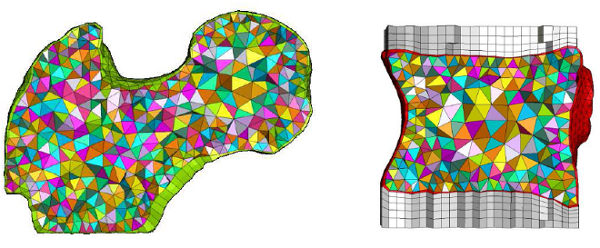
This mesher is designed to mesh thin layers (e.g. cortex) and produces flat elements. In case of other topologies maybe different meshers (e.g. CGAL 3D mesher) are more robust and easier to use.
The initial surface can be triangulates (‘tria’ version) or meshed with quadrilateral elements (‘quad’ version): In the ‘tria’ version the solid region which is covered by the thin layer is meshed by using GMSH (http://geuz.org/gmsh/) which is not part of medtool. Executables from external resources are added for different platforms without any warranty. Gmsh can to be compiled and installed elsewhere and linked to the script with the ‘exe’ option.
In case of the quadrilateral elements (‘quad’ version) a corresponding linear hexahedral mesh of the solid region (trabecular volume) can be provided (‘vol’ option). In this case the spongious region will be adopted (refined in case) and only the cortex will be meshed.
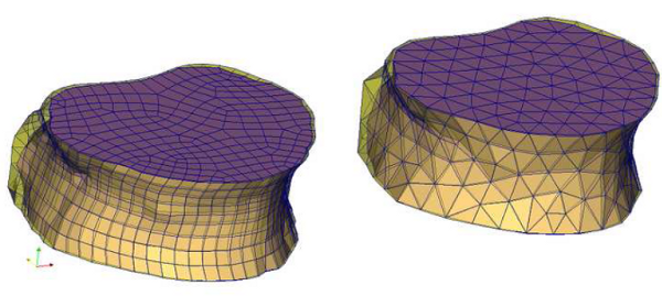
The initial surface should be rather coarse and close to the voxel thickness images. It can be refined by the mesher (‘refi’ option). This makes the algorithm much more robust. Each refinement level reduces the edge length by a factor of two and is done in a way that crossing normals are avoided.
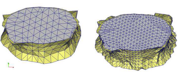
The given contour should be close to the given voxel thickness information. It can be modified in the following ways :
translate (‘tra’ option) and scale (‘sca’) initial surface
equivalence nodes (‘equi’) i.e. stitch of initial surface
find holes in surface - only checked and reported, not repaired
flip the initial surface normals (‘flip’) and output the flipping.
However, it is recommended to use graphical tools like Paraview or FE pre-processors (e.g. Hypermesh) to check and repair the isosurface as well as to see if the voxel image and isosurface fit. In the current version the offset of the voxel image is not implemented and the voxel image is assumed to start at 0,0,0. A limited information about the bounding boxes is given for a rough check.
The basic idea of the algorithm is straight forward. A ray (line) starts at the isosurface ‘s’ and walks in the normal direction ‘–>’ of this surface to find intersections ‘i’ between the ray and the voxel thickness information ‘x’ (voxels are modelled as cubes).
Graphically this means
voxel thickness       0s000000xxxxxxxxxxxxxxxx00000000000
ray along normal       --->--i-->-->-->-->-->-i
result of algorithm          |<-  Thickness ->|

                      s...isosurface postion, x...cortex voxels,
                      0...marrow voxels,      i...intersections,
                      --> ... travel direction
This obtained information is used to :
move the isosurface from point ‘s’ to the first intersection ‘i’ and
to construct a solid element between the two intersections ‘i’.
Practically several points must be considered to obtain a correct thickness. In the first step, the algorithm computes averaged normals at each node of the isosurface based on the normals of the surrounding elements. If the sharp feature meshing is active at the boundary (‘adj’) the algorithm checks the COG of the isosurface elements with respect to the distance to the boundary. Whenever the distance is smaller than ‘adj’ no solid element is generated at the boundary and normals are adjusted at the boundary such that they are within in the section plane (for more details see ‘adj’ option).
After the computation (adjustment) of the normals, the thickness of each node is computed by walking from outside or inside (‘dir’ option) along the previously computed (maybe adjusted) normals. The convention is that the normals of the given surface have always to point outwards in both cases. The ‘dir’ options selects the walking direction based on this assumption. If ‘isosurf’ is used the normals are fine. In case of the CGAL mesher they need to be checked and maybe flipped.
Because the isosurface is never exactly at the voxel thickness image, an ‘start’ position should be provided (see ‘start’ option). The ray starts the search not at the isosurface but with an offset given by this distance. A file with the name ‘test-start_pt-normal.case’ is written and shows the start points and the walking direction.
The finds the exact start and end points where a ray intercepting the voxel cubes. Small holes and single voxel hits are avoided by given proper parameters in ‘thick’ option.
The thickness is set to the a given minimum thickness if no valid thickness can be found. A thickness is not valid if
no intersection is found
only on intersection is found
the distance between two intersections if bigger than maximum allowed thickness
In case of section models the mesh is checked for inflated elements at the boundary. Look in file ‘test-inflated-elems.case’ to see them. If inflated triangle appear the old nodal positions are there, where the element was still ok.
In summary before thickness extraction at least a:
a minimum and maximum allowed cortex thickness have to be provided (‘thick’)
a search start point offset has to be defined (‘start’)
full and section models option can be selected (‘adj’)
a coarse mesh can be refined (‘ref’) several times (more stable than an initial fine mesh)
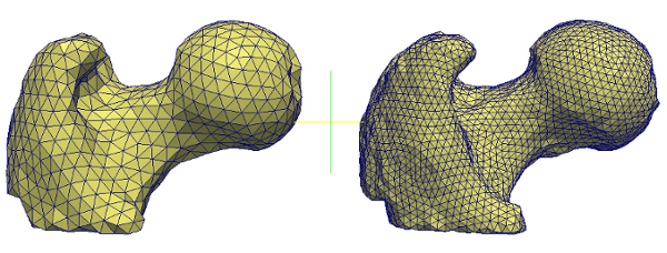
During writing of the meshing the element volume is checked. Elements with zero volume are not written. Zero volume elements is obtained if the minimum thickness is set to zero or if ‘adj’ is on. In the latter case elements at the section plane (boundary of the voxel model) have zero volume and are not written to the output.
Based on the generated cortex mesh, an the inner volume is meshed by gmsh using tetrahedrons. The computed bone meshing can be controlled via following options:
linear or quadratic solid elements (‘order’)
mesher parameter for the trabecular region (‘clmax’)
Finally volume statistics and info’s could be printed in order to be able to see the differences in the volume of the smooth mesh and voxel model.
What should I do if I have problems?
!!! R E A D this documentation C O M P L E T E L Y !!!
It is important to understand the idea behind the mesher to get an idea of the required and correct parameters.
Negative Jacobian warnings during meshing always indicate problems. Please think also about the output with ‘!!’ in front. These warnings may be OK but could also be indicators for errors.
During meshing all nodes are projected exactly at the voxel model i.e. problems of the voxel based thickness extraction are directly visible in the generated meshes.
Steps during checking could be:
Carefully read the output of the script i.e. bounding box info, Warnings, etc.
Check the initial iso-surface. Display the normals (have to point outwards), look for holes, unconnected regions, and mesh distortions with a separate tool like Paraview (www.paraview.org) or HyperMesh.
Generate an Ensight file from the thickness voxel model for Paraview (mic->’.inp’ and fec->’.case’). Note that the ‘.mhd’ file is shifted and smaller than the internally used voxel model (due to VTK conventions). But for a quick check it could be also used.
Load the starting surface in Paraview. The scaled and translated surface is written to a file named ‘filename’_start_2Din.case or ‘filename’_start_2Dout.case.
Load the start postions and directions from file ‘test-start_pt-normal.case’
Check the computed 2D surfaces ‘filename’_2Din.case or ‘filename’_2Dout.case. These surfaces are move exactly to the voxel model! Especially look if at nodes with min/max thickness.
Check the extracted normal and thickness ‘filename’_Norm.case.
Usage
Command line:
python bom.py ...

  -inv       voxFilename
  -ins       surfFilename
  -out       meshFilename
  [-vol]     meshFilename                             (optional)
  -dir       directions
  [-mout]    meshOutType                              (optional)
  [-sca]     scaleFactor                              (optional)
  [-tra]     move1;move2;move3                        (optional)
  [-equi]    phyDistance                              (optional)
  [-flip]    filename                                 (optional)
  [-eflip]   featureAngle                             (optional)
  -thick     phyMinThick;phyMaxThick
  -start     phyDistance
  [-correct] phyThickness                             (optional)
  [-corrfkt] filename                                 (optional)
  [-nomin]   flag                                     (optional)
  [-adj]     phyTolerance                             (optional)
  [-ref]     level                                    (optional)
  [-order]   meshOrder                                (optional)
  [-ncort]   number                                   (optional)
  [-exe]     filename                                 (optional)
  [-clmax]   maxCellSize                              (optional)
  [-stat]    voxOutsurfFileName                       (optional)
  [-ifo]     fileName;mode                            (optional)
  [-help]                                             (optional)
Parameters
- -inv
: voxFilename
Image data input file where thickness information is stored which includesalso physical dimensions (e.g. like a ‘.mhd’ file).
- -ins
: surfFilename
Input file where the inner or outer surface is stored. This isosurface can be given in any dimensions. Use ‘sca’ to scale the surface and ‘tra’ to translate the surface if necessary. If the surface is in physical dimensions a scale is not necessary. It is important that the surface and the voxel fit together i.e. have same physical dimensions. The mesh can be a tria mesh or quad mesh (only together with ‘vol’ option). Note: Normals have always to point outwards!
- -vol
: meshFilename
Inner linear hexahedral volume mesh. If this option is given following points should be considered:
‘dir’ is set to inside internally
the trabecular region will not be meshed ‘clmax’ will be ignored but order changes are possible
the ‘ins’ has to provide a conform 2D quad mesh which covers the whole volume. Tria’s are not tested.
nodes of the 2D and 3D mesh will be automatically equivalenced ‘equi’ is automatically performed.
‘flip’ is not working - use surfaces where normals point outwards
‘eflip’ is not working - only for triangles
meshes from cubit are tested e.g. follow ‘jou’ can be used to generated both meshes
## /usr2/pahr/software/cubit11.1/bin/clarox
## Cubit Version 11.1
## Cubit Build 38921
## Revised 2008-12-12 10:55:21 -0700 (Fri, 12 Dec 2008)
## Running 12/21/2008 10:19:03
## Command Options:
## -warning = On
## -information = On
import stl "surface_in.stl" feature_angle 135 linear merge
volume 1 size 8
volume 1 scheme sweep source surface 2 target surface 3 rotate off
volume 1 sweep smooth auto
mesh volume 1
block 1 volume all
export abaqus "hexa_mesh.inp" block 1 overwrite
block 2 surface all
export abaqus "quad_mesh.inp" block 2 overwrite
- -out
: meshFilename
Output file name where the meshes are written. Currently 2D inner/outer surface and 3D spongious/cortical volume meshes are written to the output. In case of Ensight file output also the normal normal directions are written.
- -dir
: direction
Indicate the moving direction of the algorithm e.g. if the surface is the inner or outer surface. Normals has to point outwards in both cases. ‘direction’ can be ‘out’ or ‘in’. ‘in’ means you are running from inside to outside.
- -mout
: meshOutType
Limited mesh output. The parameter can be ‘S’ for 3D sponge mesh ‘C’ for 3D cortex mesh, ‘B’ for both 3D meshes, 2D for 2D meshes and normals only and B+2D for both. If this parameter is not given both meshes are written to the output (B+2D).
- -sca
: scaleFactor
Multiplication which is applied on each point of the surface to scale the surface in the correct physical dimension. Usually it is the resolution where of the voxel model which is used to extract this surface.
- -tra
: move1;move2;move3
Translation of the surface in 1,2,3 direction. The distance have to be provided in physical dimensions. E.g. isosurf surfaces need a translation of lenVox/2.
- -equi
: phyDistance
Physical equivalence distance. This parameter is used if mesh patches of the surface should stitched together. This is done by equivalencing nodes. Currently only simplex surfaces are implemented (one close surface). If holes/unconnected regions are detected this option tries to stitch the surface
- -flip
: filename
Flip the normals of the input surface such that the normals point outwards. Afterwards the result is written to ‘filename’ to be able to check them.
- -eflip
: featureAngle
Flip the edges of the initial triangular surface file. It checks the element quality of two adjacent triangle before and after a possible flip. If the quality is increase the edges will be flipped. Furthermore the angle of elements normals is checked. If the angle is smaller than the “featureAngle” the edges are allowed to be flipped.
- -thick
: phyMinThick;phyMaxThick
These parameters are needed by the thickness extraction algorithm (see above) and has to be given in physical dimensions. A minimum and maximum thickness have to be provided.
The minimum thickness has three influences:
It is used during thickness computation. If no valid thick could be found this thickness is used instead. No valid thickness are e.g. in case of the to small maxThickness (see below) or when a ray do not find two intersections (only start but no end voxel is found), or if whether a start nor end is found. If minThick=0.0 element edges will be collapsed. This might be problematic in case of FEA.
Second this parameter is used in after the thickness extraction to correct the meshes. If an element with volume>0 but possible zero thickness at one location of node pairs, this thickness will be used to avoid collapsed edges.
Third, if all nodes have a zero thickness than this thickness is used and used for the calculation of the element volume. The output of this element can be controlled with the ‘wrmin’ option. If the option is ‘ON’, this element is not written and holes become visible.
The minimum thickness is automatically set to zero in case of section bone models (‘adj’ on) for elements at the boundary.
The maximum thickness gives the maximum allowable cortical shell thickness and has influences on the search algorithm. This parameter is necessary to overcome problems with small holes in the cortex as well as single voxel thickness due to the digitization. Example with small holes
Cortex Hole Cortex Trabecular Other Cortex \ / / / / Voxel Ray: 00000xx00xxxxxxxxx000000000000000000xxxxxx0000 |<-Thickness->| |<- maxThickness ->| x...cortex voxels, 0...marrow voxels 'Thickness' is the obtained quantitiy Note: Do not make maxThickness to big otherwise the opposite cortex will be included i.e. a wrong thickness will be detected! - Example: |<- Thickness ->| |<- maxThickness ->| 00000xx00xxxxxxxxx000000000000000000xxxxxx000000 Do not make maxThickness to small. Otherwise - Example: detected thickness is "3"! |<->| Thickness |<- maxTh ->| 00000xxx00xxxxxxxxx000000000000000000xxxxxx000000 - Example: detected thickness is minimum Thickness because no valid intersection is found. |<-Thickness->| |<- maxTh ->| 00000xxxxxxxxxxxxx000000000000000000xxxxxx000000- -start
: phyDistance
This is a physical distance (offset) where the start should begin. Search start points are the nodal positions of the isosurface plus a physical distance given by this option. If this distance is 0 or not given the start point are the nodal positions. In some cases this may lead to errors. Therefore, this offset can be given by the user. If start points are in the cortex or outside the voxel model warnings will be printed (output starts with ‘!!’ ). If the offset and surface is correct than this output will be suppressed. The start points and start normals are written to an Ensight Gold File named ‘test-start_pt-normal.case’ and can be checked with Paraview. Be careful when choosing this distance to small. It will produce nodes with minThickness i.e. always check if the number of nodes with minThickness change if this parameter is increased! If the distance is too big than the start point could be outside of the voxel image and it needed to be covered with ‘0’ voxels such that the start point is inside the voxel model (e.g. using ‘mic’).
Graphical explanation (Case isosurface in cortex, search from outside to inside)
start positio   Cortex  isosurface    Cortex         Inside
      \             \    /            /              /
0000000s000000000000xxxxixxxxxxxxxxxxxxxxxxxxxxxxx0000000000
       |<-    start   ->|
For example, if the isosurface is always outside (or inside) of the cortex this distance can be given as zero.
- -correct
: phyThickness
Correction parameter for the detected thickness. Currently this is a global correction and do not take curvature etc. into account. The parameter ‘pythThickness’ is the amount of physical distance which is added to the detected thickness. It controls mainly the cortex volume. Always look at ‘stat’ option to check the volumes.
- -corrfkt
: filename
Function which is applied to correct the computed thickness values. The function is provided in an python file. The computed thickness by the algorithm has the variable name “thickOld” and the returned variable with the corrected thickness has the name ‘thickNew’. The evaluation is done after the thickness computation. Thus it’s a simple post-processing step. Again two variables are predefined :
thickOld … the internal computed thickness by this routine
thickNew … the corrected thickness
Example
thickNew = 1.2 * thickOld + 0.08
Also a simple python code fragment can be used to model more complex corrections. Please note the python syntax (indentation and linefeed) has to be written correctly.
- -wrmin
: flag
This flag controls if elements with minimum thickness at all nodes are written to the output or not. If this flag is not given or is set to ‘OFF’ such elements are not written. If the flag is ‘ON’ elements with a minimum thickness at all nodes are written. Before switching this option “ON” it is recommended to run the mesher with the flag ‘OFF’ first in order to check if holes appear in the cortex.
- -adj
: phyTolerance
This parameter is used to mesh section models. Normals at the boundary are adjusted properly. The provided value is the search tolerance in physical dimensions to locate nodes at the boundary. If it is zero or not given nodes will not be adjusted. If this parameter is given:
the normals are not smoothed over the boundary
the normals are adjusted for nodes at the boundary (projected to the plane at the surface)
The value of this option can be simply evaluate by looking at the bounding box output. Be careful when choosing this value. If it is to big it might pull nodes from the cortex to the boundary!
- -ref
: level
Mesh refinement level. After the first normal/thickness detection the mesh is refined and the normal/thickness as well as position of the new nodes are computed. This parameter specifies how often a mesh refinement operation should be performed. Compared to the initial thickness detection, the normals during the refinement level are not computed form the mesh but interpolated from the initially detected normals. This strategy is more robust because newly generated nodes are always in between old ones. Important is that the thickness detection of the coarse mesh show no problems. If this parameter is given as ‘0’ no refinement will be done.
- -order
: order
Order of the produced meshes 1 or 2 i.e. linear or quadradic meshes are written. This options makes only sense if Abaqus files (‘.inp’) files are written. Default is 1.
- -ncort
: number
Number of cortex elements over the thickness. 1 or 2 elements are possible. Default is 1.
- -exe
: filename
Path to Gmsh executable. If not given, an executable named ‘gmsh’ will be called from the MEDTOOLPATH directory. The selected mesher/optimizer is netgen.
- -clmax
: maxCellSize
Mesher parameter. Maximal allows mesh size. If this parameter is not given the mean nodal distance of the surface mesh will be used.
- -stat
: filename
This is the image data (voxel model) of the outer surface and should correspond with the image data for the thickness. It is used in ‘ifo’ option to compute the total volume of the bone.
- -ifo
: filename;mode
Write volume and surface statistics to a file. If a file name is given the computed info is written to the file. The “mode” can be “w” (create new file, write header + data in single line), “a” (append to file, write data in single line) or “f” (write a full output). This option needs the ‘stat’ option to compute the volume of the bone.
- -help
: Print usage
Info
File: bom.py
Author: D.H. Pahr
3D - GMSH
This script allows using gmsh to create and modify finite element meshes.
Usage
Module:
import gmshMesher
Command line:
python gmshMesher.py ...

   -inf      testIn.stl
   -outf     testOut.inp
  [-tetfill  maxElementSize;newElsetName   ]
  [-exe      path                          ]
  [-doc                                    ]
  [-help                                   ]
Parameters
- -inf
: filename
Reads a mesh with filename ‘filename’. The file type is a recognized by the extension: Possible extensions are:
‘inp’: ABAQUS input file. Implemented keywords:
*HEADING
*NODE
*ELEMENT
*NSET
*ELSET
‘.off’: Geomview (only triangles implemented)
‘.msh’: Gmsh mesher
‘.vtk’: vtk ASCII file
‘.stl’: stereolithography file
‘.obj’: wavefront obj file
‘.fem’: Nastran/Optistruct file
- -outf
: filename
Writes a mesh with filename ‘filename’. Possible types are:
‘.geo’: PARAVIEW : Ensight gold format (same as ‘.case’)
‘.case’: PARAVIEW : Ensight gold format (same as ‘.geo’)
‘.inp’: ABAQUS input file
‘.msh’: GMSH file
‘.vtk’: vtk ASCII file
Optional Parameters
- -tetfill
: maxElementSize;newElsetName
Fills a given triangular surface mesh with tetrahedral elements. ‘maxElementSize’ is the maximum element size of the internal elements. The surface mesh remains unchanged. ‘newElsetName’ is the name of the newly generated tetrahedral mesh.
- -exe
: path
Path or command to the gmsh executable. By default, the command ‘gmsh’ is used.
Info
File: hma.py
Author: D. H. Pahr
Converter
Script converts different unstructured grid (FEM) file formats. Implemented grid elements which can be read and write are:
bar2
bar3
tria3
tria6
quad4
quad8
hexa8
hexa20
pyra5
penta6
penta15
tetra4
tetra10
Meshes can be refined, smoothed, cropped, translated and elset can be extracted.
Usage
Module:
import fec
Command line:
python fec.py ...

  -in         filename
  -out        filename
  [-bin]      flag                                   (optional)
  [-bbcrop]   start1;start2;start3;end1;end2;end3    (optional)
  [-extr]     setname                                (optional)
  [-refin]    flag                                   (optional)
  [-order]    order                                  (optional)
  [-smooth]   type;niter;[param2];[param3]           (optional)
  [-latt]     thickness                              (optional)
  [-tra]      tra1;tra2;tra3                         (optional)
  [-tfil]     filename                               (optional)
  [-texp]     exponent                               (optional)
  [-histo]    filename;errorVal;normalize;nIntervals (optional)
Parameters
- -in
: filename
Name of the file which is to be converted. The file type is a recognized by the extension: Possible extensions are:
‘inp’: ABAQUS input file. Implemented keywords:
*HEADING
*NODE
*ELEMENT
*NSET
*ELSET
‘.raw’: ASCII file from dualcontour program
‘.off’: Geomview (only triangles implemented)
‘.msh’: Gmsh mesher
‘.vtk’: vtk ASCII file
‘.stl’: stereolithography file
‘.obj’: wavefront obj file
‘.fem’: Nastran/Optistruct file
- -out
: filename
Name of the result files, converted file. Possible types are:
‘.geom’: TAHOE II format
‘.geo’: PARAVIEW : Ensight gold format (same as ‘.case’)
‘.case’: PARAVIEW : Ensight gold format (same as ‘.geo’)
‘.inp’: ABAQUS input file
‘.off’: Geomview file
‘.msh’: GMSH file
‘.stl’: stereolithography file
‘.surf’: netgen’s surface mesh file
‘.smesh’: tetgen’s surface mesh file
‘.vtk’: vtk ASCII file
- -bin
: flag
Toggles writing binary STL files ‘ON’ or ‘OFF’.
-props : flag
Reads Material in case of Abaqus inp files .
- -bbcrop
: start1;start2;start3;end1;end2;end3
Output only a part of the model which is inside the given bounding box given by ‘start1’, ‘start2’, ‘start3’, ‘end1’, ‘end2’, ‘end3’. The COG of the elements are used to define what is inside. Parameters are the start and end points of the bounding box in physical dimensions.
EXAMPLE :
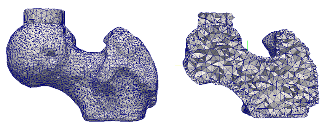
- -extr
: setname
Extracts a mesh from a given elset name ‘setname’.
EXAMPLE :
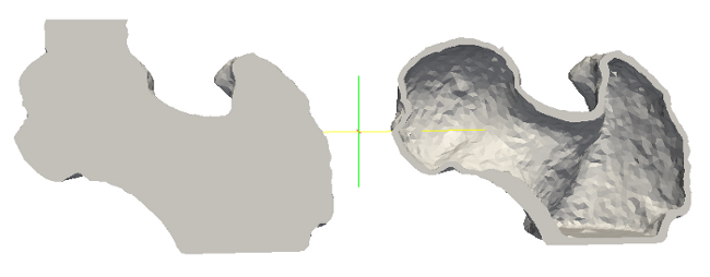
- -refine
: flag
If the ‘flag’ parameter is set to “ON” the mesh will be refined. Only linear meshes will be refined.
EXAMPLE :
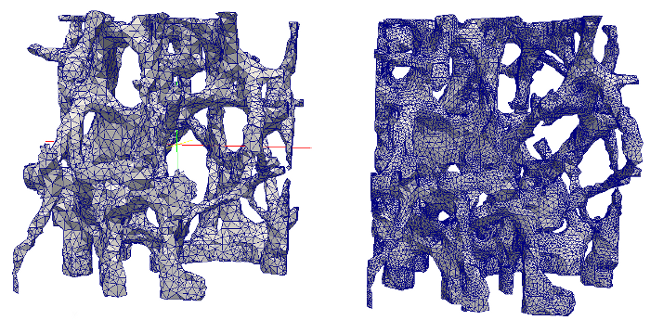
- -order
: order
Order of the mesh. This function converts linear to quadratic meshes. or quadratic to linear meshes. Allowed values for ‘order’ are 1 or 2. Currently only 1st to 2nd order change is implemented. The nsets are not modified by this function. Quadradic output is only fully supported for ABAQUS and ENSIGHT (Paraview).
- -smooth
: type;niter;[param2];[param3]
Smooth the mesh. Currently only triangulated meshes (tria3) can be smoothed. Laplacian and Taubin smoothing are possible.
Possibel ‘type’ values are:
‘Laplace’ for Laplacian. where ‘niter’is the the number of iterations. ‘param2’ and ‘param3’ are not needed.
‘Taubin’ for Taubin smoothing. where :
‘niter’ = is the number of iterations
‘param2’ = lam which is the scaling factor lambda (0<lambda<1)
‘param3’ = kPB which is the pass-band frequency kPB
Note that kPB = 1/lambda + 1/mu > 0). The implementation follows Taubin’s algorithm (see, Taubin, Eurographics 2000, Boyd and Mueller 2006).
- -latt
: thickness
Extract the lattice structure of the given 1D, 2D, or 3D mesh. The ‘thickness’ is given via the input.
EXAMPLE :
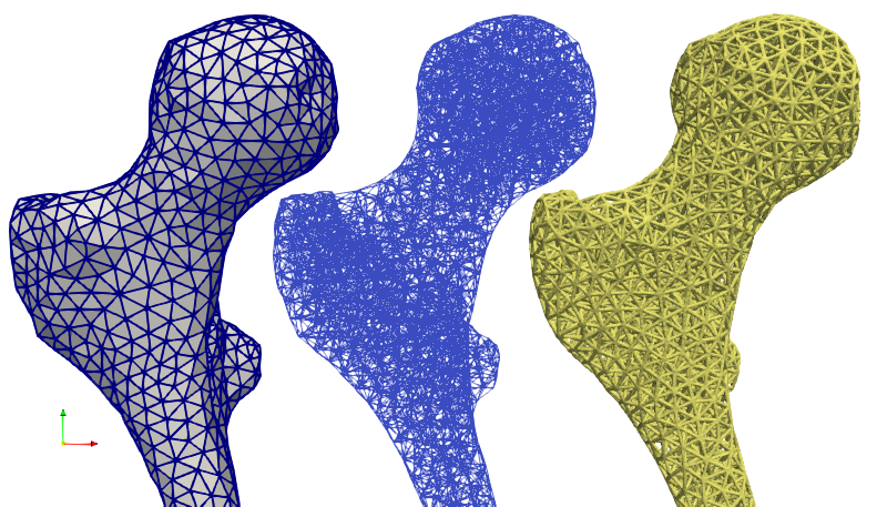
- -tra
: tra1;tra2;tra3
Translation of nodes in x,y,z (1,2,3) direction. This is the same as ‘space origin’ or ‘offset’ in image files. This parameter is ignored on case of ‘tfil’ option because there the movement comes directly from the transformation file.
- -tfil
: filename
Transform nodal coordinates by using the information given in a transformation ‘filename’. Implemented file formats are:
‘tfm’: ITK transformation file. For example, exported from 3D Slicer. The important informations in this file are ‘Parameters’ which gives the transformation matrix and ‘FixedParameters’ which gives the offset. The ordering of ‘Parameters’ is
11 12 13 21 22 23 31 32 33
and differes from the ‘nhdr’ and ‘mhd’ order scheme. The information is stored in ITK style an could be directly used in an ITK resampling filter. Compared to a classical forward transform (from input space to output space) the given transformation matrix inside this file maps points from the output space (world or new space) back to the input space (measurement or old space). This is known as backward transform. The forward transform is obtained by appling the inverse of the transformation matrix.
‘nhdr’: NRRD image header file with transformation information in it. The important informations in this file are ‘space directions’ which gives indirectly the transfromation matrix and ‘space origin’ which gives the offset. The transformation matrix is obtained from ‘space directions’ by normalizing it because ‘space directions’ include the voxel length! The ordering of ‘space directions’ is
11 21 31 12 22 32 13 23 33
The transformation matrix inside this file maps points from input space (measurement or old space) to output space (world or new space). This is known as forward transform. The backward transform is obtained by appling the inverse.
‘mhd’: ITK meta image header file with transformation information in it. The important informations in this file are ‘TransformMatrix’ which gives the transfromation matrix and ‘Offset’ which gives the offset. The ‘CenterOfRotation’ has to be (0,0,0). Non zero center of rotations are not implemented. The ordering of ‘TransformMatrix’ is
11 21 31 12 22 32 13 23 33
The transformation matrix inside this file maps points from input space (measurement or old space) to output space (world or new space). This is known as forward transform. The backward transform is obtained by appling the inverse.
The implemented transformation are based on following theoretical background. Measurements are given in a basis M and should be transformed to a basis B. These are give by unit vectors namely
b_i: unit vectors of world space basis B (new basis). This is usually b_1= (1,0,0), b_2=(0,1,0), b_3=(0,0,1).
m_i: unit vectors of measurement basis M (old basis) which are given in cooradinates measured in basis B. For example, a counter-clockwise rotation of 30 deg around the 3-axis gives m_1 = (0.866, 0.5, 0.0), m_2 = (-0.5,0.866,0.0), m_3 = (0, 0, 1).
The corresponding transformation matrix is given by the dot product indicated by a point ‘.’
       | b_1.m_1  b_1.m_2  b_1.m_3 |   | T_11  T_12  T_13 |
T_BM = | b_2.m_1  b_2.m_2  b_2.m_3 | = | T_21  T_22  T_23 |
       | b_3.m_1  b_3.m_2  b_3.m_3 |   | T_31  T_32  T_33 |
and to transform a vector v measured in basis M denoted as [v]_M into [v]_B ie. vector v measured in B it holds
[v]_B = T_BM . [v]_M
the back-transform is given by the inverse
[v]_M = T_BM^(-1) . [v]_B
These relations are written in homogenous coordinates as
| v_1 |     |  T_11  T_12  T_13  t_1  | | v_1 |
| v_2 |   = |  T_21  T_22  T_23  t_2  | | v_2 |
| v_3 |     |  T_31  T_32  T_33  t_3  | | v_3 |
|  1  |_B   |_  0     0     0     1  _| |  1  |_M
In this way translations (tra can be realized. Note that the translation vector is given by the file and not taken from the ‘tra’ option.
- -texp
: exponent
Transformation exponent. Possible choices are
‘1’ forward transform
‘-1’ backward transform
in case of vectors this means (see option ‘tfil’)
[v]_B = T_BM^( 1).[v]_M     (forward)
[v]_M = T_BM^(-1).[v]_B     (backward)
- -histo
: filename;errorVal;normalize;nIntervals
Output histogram for the specified “errorValue”.
‘filename’ where the computed info is written.
‘errorVal’ error value. Implemented values are:
‘ar’ : edge aspect ratio of min/max edge length
‘normalize’ option. Can only have the values ‘y’ or ‘n’. If ‘y’ the percentage of volume within the interval instead of the number of voxel will be given.
‘nIntervals’ number of intervals, if not given, the interval size will be “1”.
- -help
: Print usage
Info
File: fec.py
Author: D. H. Pahr
Material
Computational homogenization is a method to model hierarchical materials. Information of a micro-structural level is used to compute an equivalent stiffness and strength which is used in macroscopic models.
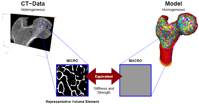
This information has to be computed and mapped from CT images to Finite Element material cards. medtool supports Abaqus/Calculix and Ensight ‘.case’ (Paraview) format.
CT Interpolator
The script performs multiple morphological analyses based on ROIs from CT images. ROIs are automatically cropped and bone densities as well anisotropy is computed over a whole micro-structure of a bone. Such maps can be visualized as shown in the following figure.
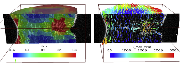
Additionally, homogenized material cards (isotropic or anisotropic) can be written for finite element analyses based on the density and fabric quantities.
Computed values are interpolated for each finite element based on a rectangular background grid as shown in the following.
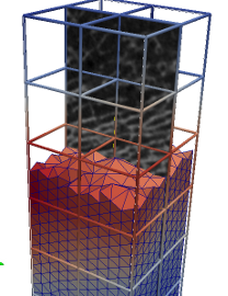
Possible material cards are:
isotropic: power law model based on CT density information
orthotropic: density based fabric or GST elasticity relationship based on CT density and fabric or GST information.
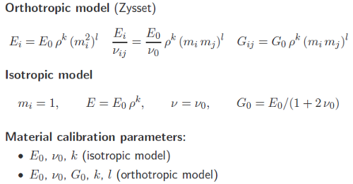
More details are given in:
Pahr, D. H. & Zysset, P. K. J Biomech, 2009, 42, 455-462
The BV/TV can be computed from a segmented or gray-level image (BMD) and calibration laws can be used. The fabric is computed from a segmented image. Usually regions are masked (e.g. cortex) to analyse one interested region per run.
Computed information can be displayed e.g. with Paraview, analysed with a spreadsheet software, or used for FE analyses.
Usage
Command line:
python  mia-multi.py ...

  -infm    filename
  -thrm    threshold
  -thrb    threshold                            [optional]
  -infs    filename                             [optional]
  -rvet    type
  -rveg    phyDistance
  -rved    phyDimension
  -morp    step;power;validLen
  -faba    fabriShape
  -fabm    morphType
  -fabn    normType
  -fgst    n;DTI;volRation                      [optional]
  -fabs    shift;slope                          [optional]
  -morf    filename                             [optional]
  -matt    model;par1;par2;...
  -bmdd    function                             [optional]
  -bvtv    function                             [optional]
  -femf    filename
  -feme    setName
  -outf    filename                             [optional]
  -outp    filename                             [optional]
  -oute    filename                             [optional]
  -outm    filename                             [optional]
  -outs    specifier1;specifier2;...            [optional]
  -outa    filename;mode;eval                   [optional]
  -outi    filename;bins                        [optional]
  -outn    nMats                                [optional]
  -run     flag                                 [optional]
  -echo    flag                                 [optional]
  -help                                         [optional]
Parameters
- -infm
: filename
Name of a masked gray value image data (voxel model). Mask means that only the interested region is visible (e.g. cortex is masked). Use ‘thrm’ to give the gray value for the mask (e.g. 0). This model is used for the BV/TV calculations and if ‘infs’ is not given it is also used for the fabric evaluations. Note: Voxels with a value of ‘thrm’ are not considered in the calculations and treated as zero volume (ZV). If you like to include regions (e.g. holes inside the bone), give them a small value > ‘thrm’ (e.g. if the image is from 0-250, give them a value of 1). This has a minor effect on the calculations, but includes these areas. Supported file formats are ‘.mhd’ or ‘.nhdr’ files. Check always if the given mask value in ‘thrm’ option corresponds with the value of the mask in this file.
- -thrm
: threshold
This threshold is used to detect the mask. Note that no voxel model gray-value of the interested regions should have this value. Otherwise BVTV calculations are wrong. The value can be any value (have not to be zero).
- -thrb
: threshold
This threshold is used to segment the voxel model given in ‘infm’. In general this value is used for BVTV and fabric evaluations. If ‘infs’ option is given it is used to compute the BVTV only. If ‘bmdd’ option is given it is used for fabric computation only. If ‘infs’ option and ‘bmdd’ is given it is not required and an error will be thrown if it is given. if ‘bmdd’ and ‘powerlaw’ is given, its not required.
- -infs
: filename
Name of a segmented (thresholded) voxel model which is used to compute the fabric. Supported file formats are ‘.raw.xml’ and ‘.mhd’. It has to be segmented and must contain zero values and values higher than zero (e.g. 0 and 1). Note that it is not checked if the file is really segmented.
- -rvet
: type
Type of the RVE (ROI) of the bone ROI which is analyzed by morphological analysis. It can be ‘sphere’ or ‘cube’.
- -rveg
: phyDistance
Distance of the background grid points for interpolation in physical dimensions.
- -rved
: phyDimension
Diameter or edge length of the ROI in physical dimensions.
- -morp
: step;power;validLength
Parameters for the morphological algorithm. ‘step’ is the distance (number of voxels) between individual rays in ray field. ‘power’ is the parameter for the computation of the number of directions on a unit sphere (=8*4^power) ‘valid’ is the smallest valid intersection length. This is option is ignored in case option ‘fabm’ = GST. If not given, the default is ‘step’=5, ‘power’=2, ‘validLen’=0.
- -faba
: fabricShape
Approximation type of the original distribution values for ‘fabricShape’ are ‘ellipsoid’ or ‘tensor2’ for an ellipsoidal or general second order approximation. This option is ignored in case option ‘fabm’ = GST. If not given, the default is ‘ellipsoid’.
- -fabm
: morphType
Morphology type of the analysis. ‘morphType’ can be MIL/SLD/SVD/GST If not given, the default = ‘MIL’.
- -fabn
: normType
Normalization of the computed fabric. ‘normType’ can be ‘trace’ (tr(m1+m2+m3)=3) or ‘det’ (det(M)=1). If not given, the default is ‘det’.
- -fcor
: flag
Correct fabric during interpolation. Background (BG) grid cells use 8 points to interpolate the fabric for an FE element or cell. Internally - if ZV/TV > 0.99 or rho < 0.003 - an isotropic fabric is set. During the interpolation steps this means some of the background grid points show an anisotropy and some are (artificially) isotropic. This may lead to less good DA results at the boundary (rho is not affected) as shown on the figure (right).
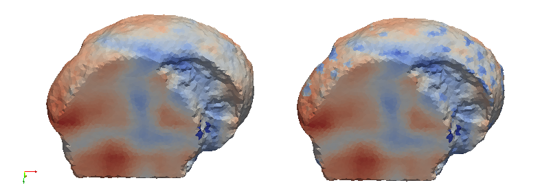
This option corrects this issue. If it is active a mean fabric is computed from those eight BG grid points which show anisotropy and the mean fabric is set to the isotropic BG grid points. The left hand side of the figure shows this corrections.
- -fgst
: n;DTI;volRation
GST parameters for the fabric. These are the power coefficient ‘n’ for the scaling of the fabric, the degree of transversal anisotropy ‘DTI’ (fabric is only considered if the computed GST ‘DTI’ is bigger than this value) . ‘volRatio’ is the ratio of curRveVol/totRveVol (only if the computed ratio is bigger than the GST is used). Isotropy is assumed if the DTI criterion or volume criterion are not fulfilled. (See Larsson et.al., Ann Biomed Eng, 2014)
DEFAULT: n=0.5:DA=1.5:zv=0.8
- -fabs
: shift;slope
These parameters give the shift and slope which should be applied on the computed fabric eigenvalues during interpolation. This can be used to transform the fabric from XCT to muCT fabric (e.g. lamMuCT_i = lamXCT_i*slope + shift). Note if shift=0.0 and slope=1.0 the fabric will be unchanged.
DEFAULT: shift=0.0, slope=1.0
- -morf
: filename
Previously computed fabric and density information is provided by a file. NOTE: All other parameters are not stored! If this option is chosen all fabric related parameters are ignored and the information is read from the file. Other parameters for the rerun are taken from the script. That means the same script should be used where this file is generate and only the ‘morph’ option is switched on.
- -matt
: type;par1;par2;…
Tissue material parameter for the density-based or morphology- elasticity relationship with
E0   ... Young's module of tissue (100% density)
mu0  ... Shear module (=G0) of tissue
nu0  ... Poisson's ratio of tissue
k    ... power coefficient for density (isotropy)
l    ... power coefficient for fabric (anisotropy)
BVTV ... bone volume over total volume (=density) between 0...1
i    ... space direction 1,2,3
m_i  ... fabric eigenvalues in i direction (EigVal1, EigVal2, EigVal3)
- Theory:
isotropic power law
E    = E0     * (BVTV)^k
E/nu = E0/nu0 * (BVTV)^k
orthotropic power law (Zysset 1995)
E_i       = E0     * (BVTV)^k * (m_i^2)^l
E_i/nu_ij = E0/nu0 * (BVTV)^k * (m_i*m_j)^l
G_ij      = G0     * (BVTV)^k * (m_i*m_j)^l
- Possibilities are:
‘zysset’;E0;nu;mu0;k,l - density-morphology based elasticity. ‘par1’=E0, …
to get eigenvalues instead of E1, E2, E3 - use zysset;1;0.3;1;0;0.5
‘powerlaw’;E0;mu0;k - density-only based elasticity. mu0 = Shear module ‘par1’=E0, …
‘powerlaw2’;E0;nu0;k - density-only based elasticity. nu = Poisson’s ratio ‘par1’=E0, …
‘user’;filename - ‘par1’ is the filename which contains the material card for the FE Solver. Following variables can be used
CardName ... material card name
BVTV     ... density
EigVal1, EigVal2, EigVal3
Formulas with these variables are evaluated using python synthax. For example (Abaqus synthax):
*material, name=CardName
*elastic
10000*BVTV**2.0, 0.3
Note: Only BVTV is evaluated, EigVal1, EigVal2, EigVal3, and CardName are only replaced.
- -bmdd
: function
If this option is activated the BVTV will be computed based on a given arithmetic function and not due to the simple threshold segmentation using ‘thrb’. A possible relation is:
BVTV = f(grayValueSum or grayValueAverage)
The internal parameter is ‘grayValueSum’ or ‘grayValueAverage’, which is the sum/average of all gray values in the considered volume element. Do not use blanks in the string or enclose the string in “..” e.g. “3 * 4” if you like to use blanks! Mask voxels are not considered in the sum/average. The two computed quantities grayValueSum and grayValueAverage are:
grayValueSum = allGrayValueSum - ZV*thrm
grayValueAverage = grayValueSum/(TV-ZV)
(TV … number of all voxel in RVE, ZV … mask voxels in RVE) If this option is not given the BVTV is computed from image given in ‘infm’. Also a simple python code fragment can be used to model more complex corrections. Please note the python syntax (indentation and linefeed) has to be written correctly. The return variable in such a python script has to be denoted as ‘newBVTV’.
- -bvtv
: function
If this option is active the BVTV will be corrected by the given arithmetic function. A possible relation is:
BVTV = f(oldBVTV)
or a python file (extension ‘.py’) with python code fragment can be provided. Two variables are predefined in this case:
oldBVTV ... the internal computed BVTV
newBVTV ... the corrected BVTV
Example :  newBVTV = 1.2*oldBVTV + 0.01
Also a simple python code fragment can be used to model more complex corrections. Please note the python syntax (indentation and linefeed) has to be written correctly.
- -femf
: filename
File where the FEM mesh is located. The mesh has to be provided in physical dimensions. Following element types are implemented: ‘tetra4’, tetra10’, ‘hexa8’, ‘hexa20’, ‘penta6’, ‘penta15’
- -feme
: setName
Name of the spongious elsets in the file given in ‘femf’.
- -outp
: filename
Name of output file where “partial” fem input information of analyzed region is written (node, elements, material cards, …). See ‘outs’ for the control of this output.
- -outf
: filename
Abaqus output file where computed material cards and other information has to be written (full output). Writes the given input file and adds the computed material cards.
- -oute
: filename
Writes information to ensight gold files (e.g. for Paraview). Following volumetric data are written
*_gridRho.*    : bone density (BVTV 0..1) at background grid points
*_femRho.*     : bone density (BVTV 0..1) at FE grid cells (elements)
*_OrientMin.*  : minimal orientation of fabric tensor atthe FE grid
*_OrientMid.*  : mid orientation of fabric tensor at the FE grid
*_OrientMax.*  : maximal orientation of fabric tensor at the FE grid
*_femDA.*      : degree of anisotropy (DA = maxEigVal/minEigVal) at FE
                 grid cells
*_femDA01.*    : degree of anisotropy (DA = 1 - minEigVal/maxEigVal) at
                 FE grid cells
*_femIsoFlag.* : indication of many grid points with DA>1 are used for
                 interpolation
Additionally a summary is written to a text file
*_femData.csv   : FE element data and some basic statistics in CSV format
*_gridData.csv  : BG grid data in CSV format
*_femData2.csv  : FE element data of stiffness and fabric orientation in CSV format
*_gridData2.csv : BG grid data of eigenvalues and fabric orientation in CSV format
- -outm
: filename
Writes the file which can be read with ‘morf’ option.
- -outs
: specifier1;specifier2;…
Output specifiers for ‘outp’ option. Implemented specifiers are:
NODE_ALL  ... write all nodes found in the 'femf' file
NODE_BONE ... write only nodes which are within 'feme' set
ELEM_ALL  ... write all elements found in the 'femf' file
ELEM_BONE ... write only elements which are within 'feme' set
NSET_ALL  ... write NSETs found in the 'femf' file
MAT_BONE  ... write material cards for the analyzed region
Default: NODE_BONE:ELEM_BONE:MAT_BONE
- -outa
: filename;mode;eval
Writes averages to an output file. ‘filename’ is a text file where the evaluation are written. ‘mode’ is the write mode (python) and can be ‘w’ for write new file or ‘a’ append on old file. ‘eval’ can be ‘f’ for fabric only or ‘fs’ for fabric and stiffness. Note that stiffness output is very slow!
- -outi
: filename;bins
Interpolate rho values (from 0…1) from background grid to an image of the same size as the input image. Results are written to the file ‘filename’. Supported formats are ‘mhd’ and ‘nhdr’. If ‘bins’ > 0, than the data are divided into intervals by the formula
value = round(rho*bins)/bins
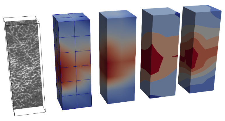
The figures shows (from left to right) the input image, the background grid values, the interpolated values with bins=0, bins=5, bins=10.
- -outn
: nMat
number of material cards in case of Abaqus power law data output. Default: 250
- -run
: flag
Controls if all background grid points should be analyzed. Can be set to ‘ON’/’OFF’. If ‘ON’ all background grid cells are analyzed. Otherwise all background grid points are detected which contain a tetrahedral bone element in it. This can yield a speed up but be careful when reading an old analysis (‘morf’ option) together with a different mesh! DEFAULT: ON
- -echo
: flag
Text output control during run. It can ‘ON/OFF’. ‘ON’ means an extended echo is written to the output screen. DEFAULT: OFF
- -help
: Print usage
Info
File: mia-multi.py
Author: D.H. Pahr
CT Direct Mapper
The script computes homogenized material cards and maps them to a given FEM model.
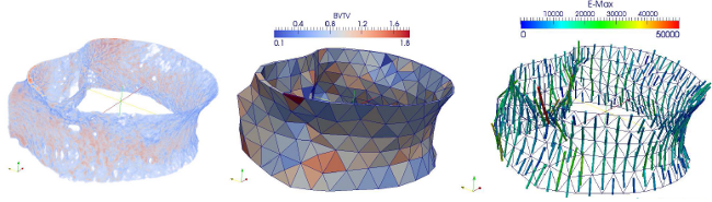
Computed values are directly mapped for each finite element based on CT values inside an FE element. Possible material cards are:
isotropic: power law model based on CT density information
orthotropic: density based fabric elasticity relationship based on CT density and global fabric information.
The BV/TV can be computed from a segmented or gray-level image (BMD). The fabric is computed from a segmented image. Regions can be masked (e.g. the cortex) but need to have a different gray value than the investigated bone region.
This script is a variant of mia-multi.py (Material - CT Interpolator). It is suggest to used the Interpolator due to efficiency and robustness.
Usage
Command line:
python  ctx-multi.py ...

  -infm    filename
  -thrm    threshold
  -thrb    threshold                                    [optional]
  -ptol    phyTolerance
  -fdir    vector1;vector2;vector3
  -fang    angle
  -frat    max;mid;min
  -fabn    fabricNormType
  -matt    model;par1;par2;...
  -bmdd    function                                     [optional]
  -bvtv    function                                     [optional]
  -femf    filename
  -feme    setName
  -outf    filename                                     [optional]
  -outp    filename                                     [optional]
  -oute    filename                                     [optional]
  -outm    filename                                     [optional]
  -outs    specifier1;specifier2;...                    [optional]
  -outh    filename;normalize;nIntervals;minVal;maxVal  [optional]
  -echo    showEcho                                     [optional]
  -help                                                 [optional]
Parameters
- -infm
: filename
Name of a masked gray value image data (voxel model). Mask means that only the interested region is visible (e.g. cortex is masked). Use ‘thrm’ to give the gray value for the mask. This model is used for the BV/TV calculations and if ‘infs’ is not given it is also used for the fabric evaluations. Supported file formats are ‘.mhd’ or ‘.nhdr’ files. Check always if the given mask value in ‘thrm’ option corresponds with the value of the mask in this file.
- -thrm
: threshold
This threshold is used to detect the mask. Note that no voxel model gray-value of the interested regions should have this value. Otherwise BVTV calculations are wrong. The value can be any value (have not to be zero).
- -thrb
: threshold
This threshold is used to segment the voxel model given in ‘infm’. In general this value is used for BVTV and fabric evaluations. If ‘infs’ option is given it is used to compute the BVTV only. If ‘bmdd’ option is given it is used for fabric computation only. If ‘infs’ option and ‘bmdd’ is given it is not required and an error will be thrown if it is given.
- -ptol
: phyTolerance
Physical search tolerance for the BV/TV computations. The provided fem elements will be extended with this physical dimension and the BV/TV will be computed within the extended element. If ptol=0.0 bvtv will be computed inside the element volume.
- -fdir
: vector1;vector2;vector3
Global direction vector which will be mapped on the cortex elements in order to give the direction of the fabric.
- -fang
: angle
If the angle of the element normal and the ‘fdir’ direction is below this angle than the fabric will be set to ‘1’ in all direction. This means isotropic material and no mapping.
- -frat
: max;mid;min
Ratio’s between the fabric directions. The first value is the global (given) direction. The third direction is in direction of the normal and the second direction is perpendicular to the previous directions.
- -fabn
: normType
Normalization of the computed fabric. ‘normType’ can be ‘trace’ (tr(m1+m2+m3)=3) or ‘det’ (det(M)=1).
- -matt
: type;par1;par2;…
Tissue material parameter for the density-based or morphology- elasticity relationship. Possibilities are:
‘zysset’;E0;nu0,mu0;k,l - density-morphology based elasticity. ‘par1’=E0, …
‘powerlaw’;E0;mu0;k - density-only based elasticity. ‘par1’=E0, …
‘user’;filename - ‘par1’ is the filename which contains the material card for the FE Solver. Following variables can be used
CardName ... material card name
BVTV     ... density
EigVal1, EigVal2, EigVal3
Formulas with these variables are evaluated using python synthax. For example (Abaqus synthax):
*material, name=CardName
*elastic
(grayValue/255.)**2.0, 0.3
- -bmdd
: function
If this option is activated the BVTV will be computed based on a given arithmetic function and not due to the simple threshold segmentation using ‘thrb’. A possible relation is:
BVTV = f(grayValueSum or grayValueAverage)
The internal parameter is ‘grayValueSum’ or ‘grayValueAverage’, which is the sum/average of all gray values in the considered volume element. Do not use blanks in the string or enclose the string in “..” e.g. “3 * 4” if you like to use blanks! Mask voxels are not considered in the sum/average. The two computed quantities grayValueSum and grayValueAverage are:
grayValueSum = allGrayValueSum - ZV*thrm
grayValueAverage = grayValueSum/(TV-ZV)
(TV … number of all voxel in RVE, ZV … mask voxels in RVE) If this option is not given the BVTV is computed from image given in ‘infm’. Also a simple python code fragment can be used to model more complex corrections. Please note the python syntax (indentation and linefeed) has to be written correctly. The return variable in such a python script has to be denoted as ‘newBVTV’.
- -bvtv
: function
If this option is active the BVTV will be corrected by the given arithmetic function. A possible relation is:
BVTV = f(oldBVTV)
or a python file (extension ‘.py’) with python code fragment can be provided. Two variables are predefined in this case:
oldBVTV ... the internal computed BVTV
newBVTV ... the corrected BVTV
Example :  newBVTV = 1.2*oldBVTV + 0.01
Also a simple python code fragment can be used to model more complex corrections. Please note the python syntax (indentation and linefeed) has to be written correctly.
- -femf
: filename
File where the FEM mesh is located. The mesh has to be provided in physical dimensions. Following element types are implemented: ‘tetra4’, tetra10’, ‘hexa8’, ‘hexa20’, ‘penta6’, ‘penta15’
- -feme
: setName
Name of the spongious elsets in the file given in ‘femf’.
- -outp
: filename
Name of output file where “partial” fem input information of analyzed region is written (node, elements, material cards, …). See ‘outs’ for the control of this output.
- -outf
: filename
Abaqus output file where computed material cards and other information has to be written (full output). Writes the given input file and adds the computed material cards.
- -oute
: filename
Writes information to ensight gold files (Paraview).
- -outs
: specifier1;specifier2;…
Output specifiers for ‘outp’ option. Implemented specifiers are:
NODE_ALL  ... write all nodes found in the 'femf' file
NODE_BONE ... write only nodes which are within 'feme' set
ELEM_ALL  ... write all elements found in the 'femf' file
ELEM_BONE ... write only elements which are within 'feme' set
NSET_ALL  ... write NSETs found in the 'femf' file
MAT_BONE  ... write material cards for the analyzed region
Default: NODE_BONE:ELEM_BONE:MAT_BONE
- -outh
: filename;normalize;nIntervals;minVal;maxVal
Output BV/TV histogram data. The ‘filename’ will be modified depending on the dataType. The ‘normalize’ option can only have the values ‘y’ or ‘n’. If ‘y’ the percentage of volume within the interval instead of the number of voxel will be given. If ‘nIntervals’ is not given, the interval size will be “10”. If ‘minVal’ and ‘maxVal’ are not given min and max will be taken from the dataset
- -echo
: flag
Text output control during run. It can ‘ON/OFF’. ‘ON’ means an extended echo is written to the output screen. DEFAULT: ON
- -help
: Print usage
Info
File: ctx-multi.py
Author: D.H. Pahr
Boundary
This module provides scripts for the computational homogenization. Example problem template for classical boundary conditions are provided. A boundary condition generation creates coupling conditions needed for the individual boundary condition types.
BCs Generator
This generator is part of a process which is able to perform unit cell analyses to compute effective or apparent stiffness tensors of heterogeneous materials.
The script takes an ABAQUS input file with *NODE definitions
and generates *NSETS as well as *EQUATIONS depending on the
chosen boundary condition. BCs type are:
SUBC … Static Uniform BC (force constrolled)
MUBC … Mixed Uniform BC (force/disp. constrolled)
KUBC … Kinematic Uniform BC (disp. constrolled)
PBC … Periodic BC
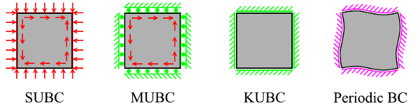
Beside internal sets for the above BCs, following sets are generated
in case of using the SET option
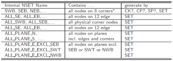
Technically following steps need to be done. Take the:
mesh from Image Processor (mic), HyperMesh, ABAQUS CAE, etc.
material, step, etc from a template file i.e. BCs Templates (cbcex)
generate the BCs (periodic, KUBCs, SUBCs, …) with this script
solve the model with ABAQUS, CALCULIX
compute the Stiffness with the Fu-Analyzer or Se-Analyzer in the Post menu.
An overview of how an FE input is generate with this script is given in the figure:
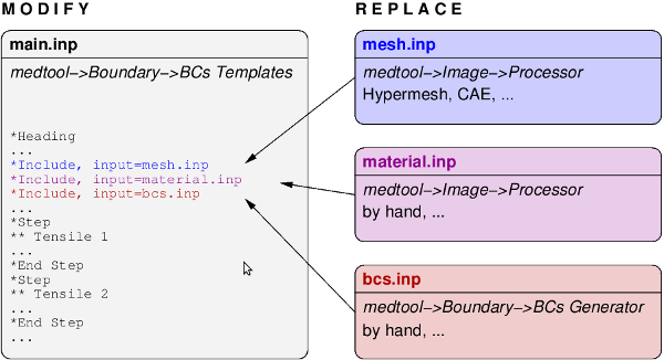
Usage
Command line:
cbc ...

  -in       InfileName
  -out      OutfileName
  -bcid     bcTypeId
  [-code]   codeName           [optional]
  [-tol]    relative tolerance [optional]
Parameters
- -in
: Name of the ABAQUS input file where the
*NODEare located.- -out
: Name of the file where
*NSETS,*EQUATIONS,etc are written.- -bcid
: Identifier for the boundary condition type. The rule is: C/S + P/K + 2/3 (e.g. C3P)
C/S … Continuum/Structural elements used
P/K … Periodic/Kinematic BCs required
2/3 … Plane (2D) or Fully (3D) periodicity
Implemented BCs are:
CP2 … continuum elems + PBC + 2D periodicity
CP3 … continuum elems + PBC + 3D periodicity
SP2 … structural elems + PBC + 2D periodicity
SP3 … structural elems + PBC + 3D periodicity
CK3 … continuum elems + KUBC + 3D coupling
- SET … write out sets for the planes, faces, edges,
and corners. These sets can be used for MUBC and SUBC
Faces, edges, and corners of the cube are denoted as
                       NWT o--------NT--------o NET
                          /|                 /|
                         / |                / |
                        WT |      T        ET |
                       /   NW       N     /   NE
                      /  W |             /    |
                 SWT o--------ST--------o SET |
                     |     |            |     |
                     | NWB o--------NB--|-----o NEB
                     |    /             |  E /
3                    SW  /    S         SE  /
|  2                 |  WB       B      |  EB
| /                  | /                | /
|/                   |/                 |/
o---- 1          SWB o--------SB--------o SEB
                  (0,0,0)
- Note: SWB has to be at (0,0,0) and fixed (DOF 1,2,3) for some
cases.
- -code
: FEM code identifier. If not given, default code is Abaqus Possible Id’s are:
‘abaqus’ … HKS Abaqus format
‘calculix’ … similar to Abaqus, for ccx solver
- -tol
: Set tolerance for classifying nodes and node pairs
- -gui
: Print GUI string on stdout
- -help
: Print usage
Info
File: cbc.cpp
Author: T. Daxner and D. H. Pahr
BCs Templates
The script writes a FEM template file based on the selected BCs and the selected FEM code. If outfileName is not given the output is written to stdout.
Usage
Command line:
python cbcex.py ...

  -bcid    bcTypeId
  -code    codeName
  [-out]   outfileName     [optional]
  [-conv]  convertFileName [optional]
Parameters
- -out
: Name of the FEM output file
- -bcid
: Identifier for the boundary condition type. The rule is: C/S + P/K/S/M + 2/3 e.g. C3P:
C/S … Continuum/Structural elements used
P/K/S/M … Periodic/Kinematic/Static/Mixed BCs required
2/3 … Plane (2D) or Fully (3D) periodicity
Implemented BCs are:
CP2 … continuum elems + PBC + 2D periodicity
CP3 … continuum elems + PBC + 3D periodicity
SP2 … structural elems + PBC + 2D periodicity
SP3 … structural elems + PBC + 3D periodicity
CK3 … continuum elems + KUBC + 3D coupling (master node)
CM3 … continuum elems + MUBC + 3D coupling
CS3 … continuum elems + SUBC + 3D coupling
Note: CM3 and CS3 are generate via the SET option as ‘bcid’ in the BCs Generator (cbc).
Faces, edges, and corners of the cube are denoted as
                           NWT o--------NT--------o NET
                              /|                 /|
                             / |                / |
                            WT |      T        ET |
                           /   NW       N     /   NE
                          /  W |             /    |
                     SWT o--------ST--------o SET |
                         |     |            |     |
                         | NWB o--------NB--|-----o NEB
                         |    /             |  E /
3                        SW  /    S         SE  /
|  2                     |  WB       B      |  EB
| /                      | /                | /
|/                       |/                 |/
o---- 1              SWB o--------SB--------o SEB
                      (0,0,0)
- Note: SWB has to be at (0,0,0) and fixed (DOF 1,2,3) for some
cases.
- -code
: FEM code identifier. Possible Id’s are:
abaqus … HKS Abaqus format
calculix … similar to Abaqus, for ccx solver
- -conv
: The content of the given file will be converted to an internal python string and written to the output file (needed for adding new template files).
- -gui
: Print GUI string on stdout
- -help
: Print usage
Info
File: cbcex.py
Author: D. H. Pahr
Solve
The solve module provids interfaces to commercial and freely available finite element solver. An efficient linear micro FE solver (ParOSol) is available for Linux.
Calculix - CCX
This script is an interface to the Calculix ccx FE Solver. CalculiX is a package designed to solve field problems using the finite element method (see http://www.calculix.de/).
The scripts takes an ‘inp’ file, runs the analysis, and creates an CalculiX ‘frd’ which can be viewed with the CGX (Calculix Graphics). Optionally a ‘vtk’ output file can be created from the scripts which can be viewed with the free software Paraview (https://www.paraview.org/).
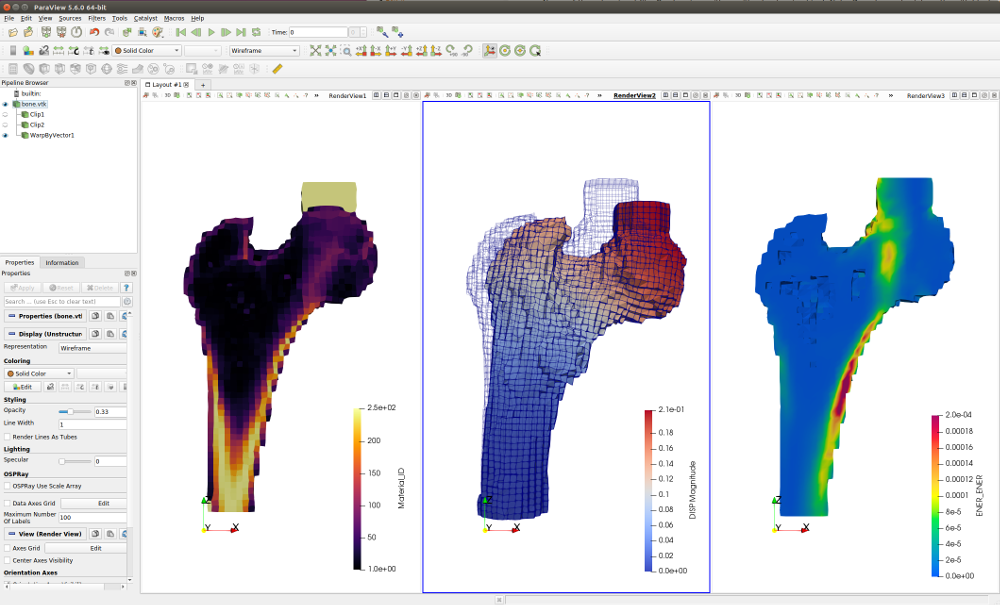
Calculix is not part of medtool. An executable from external resources is added for different platforms without any warranty. A windows version is available from http://www.bconverged.com/products.php
Notes:
Paths: It is recommended to set a working directory and use filenames without paths inside input files.
Kill analysis job: Medtool’s ‘Stop’ button do not kill the FE job! Use ‘kill’ (Linux) or the Task Manager (Windows) to kill the job!
Usage
Command line:
python ccxRun.py ...

  -inp   InputfileName
  -exe   pathToCCX       [optional]
Parameters
- -inp
: filename
Name of the solver input file. Can be given with or without extension ‘.inp’. Note: Do not use absolute paths with blanks in it! In this case choose a working directory (e.g. in medtool) with or without blanks an give the filename only.
- -vtk
: vtkFilename
Translate the ‘frd’ file to a ‘vtk’ file which can be viewed with Paraview.
- -nth
: noOfThreads
Give the number of threads which should be used by CalculiX.
- -exe
: exeFilename
Path to Calculix CCX executable. If not given, an executable named ‘ccx’ will be called from the MEDTOOLPATH directory.
- -gui
: Print GUI string on stdout
- -help
: Print usage
Info
File: ccxRun.py
Author: D. H. Pahr
Calculix - CGX
This script is an interface to the Calculix cgx pre- and post processor. (http://www.calculix.de/).
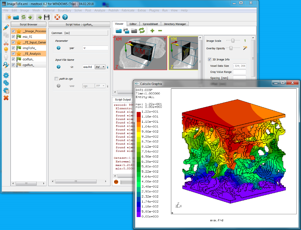
Calculix is not part of medtool. Executables from external resources are added for different platforms without any warranty. Calculix might need to be compiled / installed by the user. A windows version is available from http://www.bconverged.com/products.php .
It is recommended to set the working directory and use filenames (without paths).
Usage
Command line:
python cgxRun.py ...

  -par   parameter
  -in    filename
  -exe   pathToCGX     [optional]
Parameters
- -par
: parameter
Name of the cgx ‘parameter’ (e.g. ‘-b’, ‘-r’, etc.)
- -in
: filename
Name of model or result file. Note: Do not use absolute paths with blanks in it! In this case choose the working directory (e.g. in medtool) with or without blanks an give the filename only.
- -exe
: filename
Path to Calculix CGX executable.
- -gui
: Print GUI string on stdout
- -help
: Print usage
Info
File: cgxRun.py
Author: D. H. Pahr
Abaqus
This script is an interface to Abaqus. It starts a FE run job. (http://www.3ds.com/products-services/simulia/overview/)
Abaqus is not part of medtool. It has to be licensed, compiled, and installed by the user.
Note: Medtool’s ‘Stop’ button do not kill the FE job! Use the terminate option in this script!
Usage
Command line:
python abqRun.py ...

  -inp       inpName
  -exe       exeFilenname
  -job       jobfilename
  [-dir]     workingDirectory                 [optional]
  [-par]     par1;par2;par3...                [optional]
  [-lic]     number                           [optional]
  [-term]    flag                             [optional]
Parameters
- -inp
: filename
Name of the solver input file. Can be given with or without extension (‘.inp’).
- -exe
: exeFilename
Run command which should be used to call this script.
- -job
: filename
Name of the job filename. Can be given with or without extension
- -dir
: dirctoryName
Working directory name. In this directory, the job is run.
- -par
: par1;par2;…
Further parameters that will be added to the abaqus command. E.g. cpus=2;interactive
- -lic
: number
Script will wait until this amount of licenses given by ‘number’ are free before starting job.
- -term
: flag
If ‘YES’, the running job with the jobname defined in the parameter ‘-job’ is terminated. Nothing else is done.
- -gui
: Print GUI string on stdout
- -help
: Print usage
Info
File: abqRun.py
Author: D. H. Pahr, A. G. Reisinger
ParOSol
This script is an interface to the ParOSol FE Solver and was developed at the ETH Zuerich (https://bitbucket.org/cflaig/parosol/).
It is a fully-parallel micro-FE analysis code based on Octree to solve linear elasticity problems. Because it works on equal sized voxel geometry, it solves the problem direct on 3D images, which can be obtained by CT scans. ParOSol stands for PARallel Octree SOLver.
Usage
Command line:
python parosolRun.py ...

   -inp      inpFilename
   [-exe]    exeFilename          [optional]
   [-nproc]  noOfProcessor        [optional]
   [-par]    par1;par2;...        [optional]
   [-mpi]    mpirunExeFile        [optional]
   [-level]  multigridLevel       [optional]
   [-tol]    relativeResidual     [optional]
Parameters
- -inp
: filename
ParOSol input filename e.g. file.h5
- -exe
: exeFilename
Location of ParOSol executeable file. If not given the binary located at MEDTOOLPATH is taken
- -nproc
: nproc
Number of processors.
nproc = 1 : parosol run without mpi (default)
nproc > 1 : Parallel parosol run (called with mpirun)
If nproc >1 mpi needs to be install on the computer. Check it by type ‘mpirun’/’mpirun.exe’ in a command prompt.
- -par
: par1;par2;…
Additional mpi parameters seperated by “=”. For example ‘-par1=val1;–par2=val2’ will create: mpirun -par1 val1 –par2 val2 …
- -mpi
: exeFilename
Select a ‘mpirun’ script which is different than the machine default.
- -level
: number
Multigrid level. If not given all possible levels are used.
- -tol
: tolerance
Relative tolerance for the residual to stop the run.
Info
File: parosolRun.py
Author: D. H. Pahr
Post
The post-processing algorithm which are prived are mainly designed for computational homogenization task but can also be used for the automated reading of information from FE result files.
Abaqus - Fu-Reader
Code to reads the CF, RF, and U of selected nodes which can written to an abaqus output file.
Note: This script requires an Abaqus Python installation!
Usage
Command line:
abaqus python abqFuReader.py ...

   -odb     odbFilename
   -rpt     reportFilename
   [-exe]   exeFilename      (optional)
   [-step]  sId1;sId2;...    (optional)
   [-frame] fId1;fId2;...    (optional)
   [-inst]  instanceName     (optional)
Parameters
- -odb
: filename
Name of the FEM output database of Abaqus (ODB).
- -rpt
: filename
Name of the output file where results are written. Such an output file looks like:
XYZ; SWB;   [  0  0  0 ]
XYZ; SEB;   [  4  0  0 ]
XYZ; NWB;   [  0  4  0 ]
...
U  ; SEB:Step-1;   [ 3.0494E-03 1.8416E-13 0.0000E+00 ]
RF ; SEB:Step-1;   [ 1.0000E+00 -2.4258E-13 -6.3974E-12 ]
CF ; SEB:Step-1;   [ 0.  0.  0. ]
...
- -exe
: filename;option
This option tells the GUI that a different python interpreter should be used to call this script. Abaqus post-processing scripts require ‘abaqus python’ to be called. ‘filename’ is the Abaqus exe file which should be used and ‘option’ is a call option. For this script it is always ‘python’.
- -step
: id1;id2;…
Step ‘ids’ which should be read (default read all steps). The steps are given within double dots e.g. 2;6;7;10
-frame : id1;id2;…
Frame ‘ids’ which should be read (default frame 1). The frame are given within double dots e.g. 1;3;4;7. A further possibility is the option ‘all’.
- -inst
: name
Instance name which should be used for the evaluations. Default is ‘PART-1-1’
- -help
: Print usage
Info
File: abqFuReader.py
Author: D. H. Pahr
Abaqus - Se-Reader
This program opens an Abaqus output file and computes the stress/strain averages of an RVE. The output file is a simple text file and can be used in the SeAnalyzer to compute the homogenized stiffness matrix. In case of porous samples only the stress can be averaged i.e. -spec = STRESS has to be selected. In this case the volume average over the RVE is returned!
Note: This script requires an Abaqus Python installation!
Usage
Command line:
abaqus python abqSeReader  ...

   -in      inputFilename
   -out     outputFilename
   -size    size1;size2;size3
   [-exe]   filename;option    (optional)
   [-spec]  type               (optional)
Parameters
- -in
: filename
Finite element results file from Abaqus (ODB file) with 6 independent mechanical load cases inside. Additionally one thermal load case could be given. Step-1 – 6 are used for stiffness calculation and an optional Step-7 load case may be a pure thermal loadcase with dT=+1K!
- Note: Engineering strains are needed in the output file
(gam12, gam13, gam23 instead of eps12, eps13, eps23)
- -out
: filename
Name of the output file where stress/strain averages and porosity will be written. The Format is (last line optionial)
 ************************************************************
 *STRESS
 11 22 33 23 13 12      ** stress/strain component order
 ** LC name    S11     S22     S33    S23    S13    S12
 Step-1        13.5    34.5    0.34   0.01   0.4    -0.2
 Step-2        ...     ...     ...    ...    ...    ...
 Step-3        ...     ...     ...    ...    ...    ...
 Step-4        ...     ...     ...    ...    ...    ...
 Step-5        ...     ...     ...    ...    ...    ...
 Step-6        ...     ...     ...    ...    ...    ...
[Step-7        ...     ...     ...    ...    ...    ...]
Quantaties are volume averages.
- -exe
: filename;option
This option tells the GUI that a different python interpreter should be used to call this script. Abaqus post-processing scripts require ‘abaqus python’ to be called. ‘filename’ is the Abaqus exe file which should be used and ‘option’ is a call option. For this script it is always ‘python’.
- -size
: size1;size2;size3
This is the size of the unit cell in x,y,z. This is necessary to compute the total volume for the volume average.
- -spec
: type
Variable specifier which should be read it can be ‘STRESS’ ‘STRAIN’. If this parameter is not given both will be read.
- -help
: Print usage
Info
File: abqSeReader.py
Author: D. H. Pahr
Abaqus - Fu-Averager
Script opens an ABAQUS ‘.odb’ file and reads for a given nset the forces as well as displacements and computes the sum/average for the 1,2,3 space direction. The results are written into a text file.
Note: This script requires an Abaqus Python installation!
Usage
Command line:
abaqus python abqFuAvg.py ...

   -odb      InfileName
   -nset     NodeSetName
   -out      OutfileName
   [-mod]    outputMode       (optional)
   [-exe]    abaqusCommand    (optional)
   [-step]   stepID           (optional)
   [-frame]  frameID          (optional)
   [-mod]    outputMode       (optional)
Parameters
- -odb
: filename
Name of the FEM output database of Abaqus (ODB).
- -out
: filename
Name of the output file where averages are written. The style of such a file is
...
#odbName;step;frame;time;nset;dir_1;nData;uMean;cfMean;rfMean;uSum ...
xL2.odb;Step-1;1;0.0;ALL_NODE_T;1;1501;0.01760;0;0;26.417;0;0 ...
xL2.odb;Step-2;1;0.0;ALL_NODE_T;1;1501;-0.0049;0;0;-6.587;0;0 ...
xL3.odb;Step-1;1;0.0;ALL_NODE_T;1;1521;0.01865;0;0;28.367;0;0 ...
...
- -mod
: mode
The output for the ‘out’ option. ‘mode’ can be ‘w’ (create new file, write header + data) and ‘a’ (append to file, write data). Default is ‘w’.
- -exe
: filename;option
This option tells the GUI that a different python interpreter should be used to call this script. Abaqus post-processing scripts require ‘abaqus python’ to be called. ‘filename’ is the Abaqus exe file which should be used and ‘option’ is a call option. For this script it is always ‘python’.
- -step
: id1;id2;…
Step ‘ids’ which should be read (default read all steps). The steps are given within double dots e.g. 2;6;7;10
-frame : id1;id2;…
Frame ‘ids’ which should be read (default frame 1). The frame are given within double dots e.g. 1;3;4;7. A further possibility is the option ‘all’.
- -nset
: name
Node set which should be analyzed
- -gui
: Print GUI string on stdout
- -help
: Print usage
Info
File: abqFuAvg.py
Author: D. H. Pahr
Abaqus - Se-Averager
This script computes volume averages from integration point variables. It reads for each step/frame results and writes an xy-table. Phase averages can be obtained by using the ‘elset’ option.
Note: This script requires an Abaqus Python installation!
Usage
Command line:
abaqus python abqSeAvg.py ...

   -in       inputFileName
   -out      outputFileName
   [-exe]    exeFilename      (optional)
   [-step]   sId1;sId2;...    (optional)
   [-frame]  fId1;fId2;...    (optional)
   [-elset]  elsetName       (optional)
   -var      spec1;spec2;...
Parameters
- -in
: filename
Name of the FEM output database of Abaqus (ODB).
- -out
: filename
Name of the output file where the analysis echo will be written for the selected a step and elset. Output style
...
# V O L U M E    A V E R A G E S
# Output File : sph_sr5_PBC_NL_T_soft.out
# Step        : Step-1
# frameId frameValue       S11        S22  ..       LE11        LE22  ..
       0           0         0          0  ..          0           0  ..
       1        0.01  6.35e+07  2.558e+07  ..  0.0004998  -1.653e-08  ..
       2        0.02 1.260e+08  5.122e+07  .. -1.653e-08 -1.4481e-08  ..
...
- -exe
: filename;option
This option tells the GUI that a different python interpreter should be used to call this script. Abaqus post-processing scripts require ‘abaqus python’ to be called. ‘filename’ is the Abaqus exe file which should be used and ‘option’ is a call option. For this script it is always ‘python’.
- -step
: id1;id2;…
Step ‘ids’ which should be read (default read all steps). The steps are given within double dots e.g. 2;6;7;10
-frame : id1;id2;…
Frame ‘ids’ which should be read (default frame 1). The frame are given within double dots e.g. 1;3;4;7. A further possibility is the option ‘all’.
- -elset
: Element set name for which the averaging has to be done Default : full model
- -var
: var1;var2;…
Output variable identifier using ABAQUS conventions like
E, S, U… All components of this variable will be written.- -help
: Print usage
Info
File: abqFuAvg.py
Author: D. H. Pahr
Abaqus - History Reader
Extracts history data from an Abaqus ODB-File and writes it to ASCII-table. Notes:
First Frameement has Number 0
Needs Abaqus to run. Tested with Abaqus 6.12.1.
Script fails if Abaqus analysis was not completed.
Supports:
standard continuum elements integration point data
shell elements integration point, section point data
whole element data (e.g. whole element energy output)
node data
assembly data (e.g. energy output)
Note: This script requires an Abaqus Python installation!
Usage
Command line:
abaqus python historyReader.py ...

  -odbfile          InfileName
  -outfile          OutfileName
  [-mod]            Outputmode                     [optional]
  [-exe]            Abaqus command                 [optional]
  [-steps]          Step Name(s)                   [optional]
  [-frame]          Output Frame Number            [optional]
  [-inst]           Instance Name                  [optional]
  -set              Node- or Elementset name
  -outvars          spec1;spec2;...
  [-intpn]          Integraton point number        [optional]
  [-secpn]          Section point number           [optional]
Parameters
- -odbfile
: filename
Name of the FEM output database of Abaqus (ODB).
- -outfile
: filename
Output file name for the result output.
- -mod
: mode
Output mode for writen. ‘mode’ can be:
-‘w’…write and add 2 header lines, -‘a’…append to outfile
- -exe
: filename;option
This option tells the GUI that a different python interpreter should be used to call this script. Abaqus post-processing scripts require ‘abaqus python’ to be called. ‘filename’ is the Abaqus exe file which should be used and ‘option’ is a call option. For this script it is always ‘python’.
- -step
: id1;id2;…
Step ‘ids’ which should be read (default read all steps). The steps are given by the ‘ids’=:
‘1:2:9’ for specific steps
‘all’ for all steps in the odb file
-frame : id1;id2;…
Frame ‘ids’ which should be read (default frame 1). The frames are given by the ‘ids’=:
‘0:1:2:9’ for specific frames
‘all’ for all
‘last’ for last frame in step
- -inst
: name
Instance name which should be used for the evaluations. Default is ‘PART-1-1’
- -set
: name
Node- or Elementset name for which the data is extracted.
- -outvars
: spec1;spec2;…
Abaqus field output variables. Examples are
U1:RF3:S23… At least one Abaqus output variable must be choosen. Additional indexing variables:NR...Index Number, starting at 0 FN...odb File Name ST...Step No. FR...Output Frame No. IN...Increment No. NO...Nodenumber or Elementnumber TI...Step Time IPN...Integration Point Number SPN...Section Point Number for shell element output.
e.g.:
NR;ST;IN;NO;S22;S23;E22;E23;SDV13- -set
: name
Node- or Elementset name for which the data is extracted.
- -intpn
: id1;id2;…
Integraton point number if element output is chosen. ‘1;2;4’ for specific integration points ‘all’ for all default: ‘all’
- -secpn
: id1;id2;…
Section point number if element output is chosen. ‘1;2;4’ for specific integration points ‘all’ for all default: ‘all’
- -gui
: Print GUI string on stdout
- -help
: Print usage
Info
File: historyReader.py
Author: A. G. Reisinger
Abaqus - Field Reader
Extracts field data from an Abaqus ODB-File and writes it to ASCII-table. Notes:
First Frame has Number 0
Needs Abaqus to run. Tested with Abaqus 6.12.1
This scripts already runs on abaqus python using numpy
Output position of data:
Node set : NODAL
Element set : INTEGRATION POINT
Note: This script requires an Abaqus Python installation!
Usage
Command line:
abaqus python  fieldReader.py ...

  -odbName          InfileName
  -outfile          OutfileName
  [-mod]            Outputmode                     [optional]
  [-exe]            Abaqus command                 [optional]
  [-steps]          Step Name(s)                   [optional]
  [-frame]          Output Frame Number            [optional]
  [-inst]           Instance Name                  [optional]
  -set              Node- or Elementset name
  -outvars          spec1;spec2;...
  [-intpn]          Integraton point number        [optional]
Parameters
- -odbName
: filename
Name of the FEM output database of Abaqus (ODB).
- -outfile
: filename
Output file name for the result output.
- -mod
: mode
Output mode for writen. ‘mode’ can be:
-‘w’…write and add 2 header lines, -‘a’…append to outfile
- -exe
: filename;option
This option tells the GUI that a different python interpreter should be used to call this script. Abaqus post-processing scripts require ‘abaqus python’ to be called. ‘filename’ is the Abaqus exe file which should be used and ‘option’ is a call option. For this script it is always ‘python’.
- -step
: id1;id2;…
Step ‘ids’ which should be read (default read all steps). The steps are given by the ‘ids’=:
‘1:2:9’ for specific steps
‘all’ for all steps in the odb file
-frame : id1;id2;…
Frame ‘ids’ which should be read (default frame 1). The frames are given by the ‘ids’=:
‘0:1:2:9’ for specific frames
‘all’ for all
‘last’ for last frame in step
- -inst
: name
Instance name which should be used for the evaluations. Default is ‘PART-1-1’
- -set
: name
Node- or Elementset name for which the data is extracted.
- -outvars
: spec1;spec2;…
Abaqus field output variables. Examples are
U1:RF3:S23… At least one Abaqus output variable must be choosen. Additional indexing variables:NR...Index Number, starting at 0 FN...odb File Name ST...Step No. FR...Output Frame No. IN...Increment No. NO...Nodenumber or Elementnumber TI...Step Time IPN...Integration Point Number SPN...Section Point Number for shell element output.
e.g.:
NR:ST:IN:NO:S22:S23:E22:E23:SDV13- -set
: name
Node- or Elementset name for which the data is extracted.
- -intpn
: id1;id2;…
Integraton point number if element output is chosen. ‘1:2:4’ for specific integration points ‘all’ for all default: ‘all’
- -gui
: Print GUI string on stdout
- -help
: Print usage
Info
File: fieldReader.py
Author: A. G. Reisinger
Calculix - Se-Reader
This program opens an Calculix output file and computes the stress/strain averages of an RVE. The output file is a simple text file and can be used in the SeAnalyzer to compute the homogenized stiffness matrix. In case of porous samples only the stress can be averaged i.e. -spec = STRESS has to be selected. In this case the volume average over the RVE is returned!
Usage
Command line:
python ccxSeReader ...

   -in      inputFilename
   -out     outputFilename
   -size    size1;size2;size3
   [-spec]  type               (optional)
Parameters
- -in
: filename
Finite element results file from Abaqus (ODB file) with 6 independent mechanical load cases inside. Additionally one thermal load case could be given. Step-1 – 6 are used for stiffness calculation and an optional Step-7 load case may be a pure thermal loadcase with dT=+1K!
- Note: Engineering strains are needed in the output file
(gam12, gam13, gam23 instead of eps12, eps13, eps23)
- -out
: filename
Name of the output file where stress/strain averages and porosity will be written. The Format is (last line optionial)
 ************************************************************
 *STRESS
 11 22 33 23 13 12      ** stress/strain component order
 ** LC name    S11     S22     S33    S23    S13    S12
 Step-1        13.5    34.5    0.34   0.01   0.4    -0.2
 Step-2        ...     ...     ...    ...    ...    ...
 Step-3        ...     ...     ...    ...    ...    ...
 Step-4        ...     ...     ...    ...    ...    ...
 Step-5        ...     ...     ...    ...    ...    ...
 Step-6        ...     ...     ...    ...    ...    ...
[Step-7        ...     ...     ...    ...    ...    ...]
Quantaties are volume averages.
- -size
: size1;size2;size3
This is the size of the unit cell in x,y,z. This is necessary to compute the total volume for the volume average.
- -spec
: type
Variable specifier which should be read it can be ‘STRESS’ ‘STRAIN’. If this parameter is not given both will be read.
- -help
: Print usage
Info
File : ccxSeReader.py
Author: D. H. Pahr
Parallel FE - F-U-Reader
Script opens a hdf5 file reads ‘Fixed nodes’ (USER BC3) as well as ‘Nodal forces’ and sums/averages for 1,2,3 direction. ‘Restrained Nodes’ (USER BC1) and ‘Loaded Nodes’ (USER BC2) are not considered in the evaluations. The results are written to a text file.
Usage
Command line:
pfeFuRead  ...

      -in       InfileName
      [-out]    OutfileName          [optional]
      [-mod]    outputMode           [optional]
      [-base]   ptX;ptY;ptZ          [optional]
Parameters
- -in
: Name of the hdf5 parfe data file which should be analyzed. Note: The group ‘Solution’ have to be in the model!
- -out
: Name of the output file where averages are written.
- -mod
: The output ‘mode’ can be ‘w’ (create new file, write header + data) and ‘a’ (append to file, write data). Default is ‘w’
- -base
: Base point for the evaluation of the moments. If this parameter is avoided the base point will be 0, 0, 0.
- -gui
: Print GUI string on stdout
- -help
: Print usage
Info
File: pfeFuRead.cpp
Author: D. H. Pahr
Parallel FE - S-E-Reader
Script opens an hdf5 file reads stresses and strains and computes averages (over material id or element volume), computes failure factors (Pistoia rule), and writes output into CSV or matrix format.
Usage
Command line:
pfeSeRead  ...

      -in       InfileName
      [-out]    OutfileName                [optional]
      [-out2]   OutfileName                [optional]
      [-fail]   matid;tissueYieldVolume;tissueYieldStrain  [optional]
      [-mavg]   matid;varSpec              [optional]
      [-favg]   filename;elset             [optional]
      [-mod]    outputMode                 [optional]
Parameters
- -in
: Name of the hdf5 parfe data file which should be analyzed. Note: The group ‘Solution’ have to be in the model!
- -out
: Name of the output file where averages are written.
- -oum
: Name of the output file where only averages are written in matrix form. Only implemented for ‘mavg’ and used for the SeAnalyzer.
- -fail
: Computes the failure safety factor of linear muFE anaylsis based on the criterion of Pistoia 2002. The parameters are the material ids of the considered material region, the percentage of elements above the critical effective strain, and the critical tissue strain itself (last two in %). Material ids can be concatenate with ‘+’ e.g. 45+75+90, and < > can be used i.e. 30+>40 or <10+>50. The effective tissue strain is based on SED an directly taken from the muFE analysis. Results are written to the output file.
- -mavg
: Averages the given quantity over the different material properties (simple mean). Material ids can be concatenate with ‘+’ e.g. 45+75+90, and < > can be used i.e. 30+>40 or <10+>50. Currently implemented variable specifier (element data):
sed   ... strain energy density
sigij ... stress tensor (six components ij=11,22,33,12,13,23)
epsij ... strain tensor (six components ij=11,22,33,12,13,23)
More variable can be given at one time e.g. s11+s22+s12 This routine do not take the element volume into account nor divides the obtained quantity by a RVE volume like the ABAQUS or Calculix SeReader do.
- -favg
: Averages the given quantity over each tetrahedral element in the given finite element mesh elset, over the specified material id(s). Material ids can be concatenate with ‘+’ e.g. 45+75+90, and < > can be used i.e. 30+>40 or <10+>50. Currently implemented variable specifier (element data):
sed   ... strain energy density
sigij ... stress tensor (six components ij=11,22,33,12,13,23)
epsij ... strain tensor (six components ij=11,22,33,12,13,23)
This routine assumes same element size of all muFE elements. Currently implemented elem types: C3D4, C3D10
- -epla
: Extracts element variables from a given plane. The plane have to be specified by the direction (1,2,3), the position in this direction, and the search tolerance. All elements with COG within the tolerance are selected. Currently implemented variable specifier (element data):
sed   ... strain energy density
sigij ... stress tensor (six components ij=11,22,33,12,13,23)
epsij ... strain tensor (six components ij=11,22,33,12,13,23)
This routine assumes same element size of all muFE elements. The data are written to a text file. PARAM: dir;position;tol;specifier;filename
- -mod
: The output ‘mode’ can be ‘w’ (create new file, write header + data) and ‘a’ (append to file, write data). Default is ‘w’
- -gui
: Print GUI string on stdout
- -help
: Print usage
Info
File: pfeSeRead.cpp
Author: D. H. Pahr
Parallel FE - Xmf Writer
Scripts generates an ‘.xmf’ file which can be used to read parallel ‘.h5’ result files with paraview.
This scipts need h5dump to be installed.
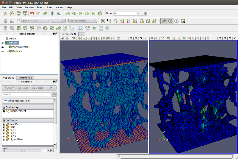
Usage
Command line:
python pfeToXmf.py ...

  -in     H5InputFileName
  -spec   spec1:spec2:....     [optional]
Parameters
- -in
: Name of the h5 file. The output file will get the same filename with the extension ‘.xmf’.
- -spec
: Variables which should be added. Implemented specifiers are:
ui   ... displacement vector (nodal data)
fi   ... force vector (nodal data)
svm  ... von Mises stress (element data)
sed  ... strain energy density (element data)
mid  ... material ids
sij  ... stress components. 'ij' can be 11, 22, 33, 12, 23, 13
eij  ... strain components. 'ij' can be 11, 22, 33, 12, 23, 13
If this parameter is not given, only the mesh is writen.
- -gui
: Print GUI string on stdout
- -help
: Print usage
Info
File: pfeToXmf.py
Author: D. H. Pahr
Fu-Analyzer
This program computes the homogenized (effective) stiffness values for a plane periodic medium (A,B,D) or spatial periodic media (E), as well as effective thermal properties if a thermal load case is given. Input values are six (or seven) independent load case. If seven load cases are given then the last one have to be a thermal load case!
Use this script in combination with any Fu-Reader.
Usage
Command line:
python FuAnalyzer.py ...

  -rpt    reportFileName
  -out    outputFileName
  -type   option
  [-prec] tolerance         (optional)
Parameters
- -rpt
: filename
Name of the file containing XYZ, U, RF, CF :
At least 6 independent mechanical load cases are required!
7 th load case may be a pure thermal loadcase with dT=+1K!
Such a file is generate with an Fu-Reader.
- -out
: filename
Name of the output file where analysis echo will be written. Example output
...
Homogenized   STRESSES
============================================================================
Step     S_11        S_22         S_33         S_23         S_13        S_12
----------------------------------------------------------------------------
1 +6.2500e-02 +8.2762e-12  +5.5626e-13  -3.7789e-14  -1.8989e-13 +2.1679e-13
2 -4.4892e-11 +6.2500e-02  -9.2731e-14  +1.9083e-14  +2.9090e-13 -3.5781e-13
3 -5.3601e-12 -1.3094e-13  +6.2500e-02  +3.3074e-15  +1.4393e-14 -1.6485e-14
4 +2.6060e-13 -4.4247e-14  -5.9446e-14  +9.2503e-14  +3.1941e-13 +6.2500e-02
5 -5.9818e-15 -3.2178e-15  +5.8056e-15  -6.2176e-15  +6.2500e-02 +3.8441e-14
6 +4.3263e-14 +1.5912e-14  +2.0401e-14  +6.2500e-02  +1.7858e-14 -3.1143e-14

ENGINEERING Constants
============================================================================
  E_1 =       81.983     |  G_23 =       16.268      | nu_23 =   -0.0046721
  E_2 =       34.261     |  G_13 =       45.377      | nu_13 =     0.085774
  E_3 =       552.55     |  G_12 =       7.8169      | nu_12 =      0.72004
- -type
: option
Type of the Periodicity, ‘plane’ or ‘spatial’
- -prec
: number
Numerical precision for checking nodal positions, differences in values of the stiffness matrix, etc.
- -help
: Print usage
Info
File: FuAnalyzer.py
Author: D. H. Pahr
Fu-Analyzer NL
This program computes the homogenized (effective) stress-strain curves for a non-linear loading of a unit cell. Output values are various stress and strain measures for different directions, as well as strain rates.
Use this script in combination with any Fu-Reader.
Usage
Command line:
python FuAnalyzerNL.py ...

   -rpt    reportFileName
   -out    outputFileName
   -type   option
   -step   id1;id2;...
   [-dir ] dir1;dir2;...  (optional)
   [-form] var1;var2;...  (optional)
Parameters
- -rpt
: filename
Name of the file containing XYZ, U, RF, CF. Such a file is generate with an Fu-Reader.
- -out
: filename
Name of the output file where analysis echo will be written. Additionally a log file will be written eg. test_log.out containing periodicity vectors, deformation gradients, etc. Example output:
...
X Y - D A T A : Hencky-Logarithmic effective STRAINS : ref=t+dt cur=t+dt
=========================================================================
Frame ij= 11 22 33 23 13 12
-------------------------------------------------------------------------
0 +0.0000e+00 +0.0000e+00 +0.0000e+00 +0.0000e+00 +0.0000e+00 +0.0000e+00
1 +2.9076e-02 -8.7223e-03 -8.7223e-03 -1.0026e-16 -6.4742e-19 +2.1935e-19
2 +5.9213e-02 -1.7763e-02 -1.7763e-02 -5.8753e-09 -1.7343e-18 +2.2643e-19
3 +9.0501e-02 -2.7148e-02 -2.7148e-02 +9.7801e-09 -1.9139e-18 +3.8588e-19
...
X Y - D A T A : Cauchy effective STRESSES : ref=t+dt cur=t+dt
=========================================================================
Frame ij= 11 22 33 23 13 12
-------------------------------------------------------------------------
0 +0.0000e+00 +0.0000e+00 +0.0000e+00 +0.0000e+00 +0.0000e+00 +0.0000e+00
1 +6.1056e+03 +0.0000e+00 +0.0000e+00 +0.0000e+00 +0.0000e+00 +1.1699e-13
2 +1.2434e+04 +0.0000e+00 +0.0000e+00 +0.0000e+00 +0.0000e+00 +1.2038e-13
3 +1.9004e+04 +0.0000e+00 +0.0000e+00 +0.0000e+00 +0.0000e+00 -7.8390e-14
- -type
: option
Type of the Periodicity. ‘option’ can be ‘plane’ or ‘spatial’
- -step
: id1;id2;…
Step ‘ids’ which should be read (default read all steps). The steps are given within double dots e.g. 2;6;7;10
- -dir
: dir1;dir2;…
Direction of additional output for xy plotting Example: 11;12;23 Available options for ‘dir’ are
'11','22','33' - normal directions
'23','13','12' - shear directions
- -form
: var1;var2;…
Formulation of additional output for xy plotting. The output will be written to a file with the same filename as given in -out but with ‘_xy_dir’ in the filename e.g. test_xy_11.out. If more then on step is requested the data will be appended. Example:
E_lin;S_lin;E_gl_tlAvailable options:'S_lin' - eff. linear/nominal stresses ref=0 'S_cau' - eff. Cauchy stresses ref=t+dt 'S_pk2_ul' - eff. PK2 stresses, update Lag. ref=t 'S_pk2_tl' - eff. PK2 stresses, total Lag. ref=t+dt 'S_ckir' - eff. corotational Cauchy str. = R^T.S_cau.R 'S_hill' - eff. Hill stresses = F^T.S_cau.F 'S_kir' - eff. Kirchhoff stresses = J.S_cau 'E_lin' - eff. linear strains ref=0 'E_log_0' - eff. Hencky/logarithmic strains ref=0 'E_log_1' - eff. Hencky/logarithmic strains ref=t+dt 'E_gl_tl' - eff. Green/Lagrange strains ref=0 'E_gl_ul' - eff. Green/Lagrange strains ref=t 'E_alm' - eff. Almansi strains ref=t+dt 'dE_gl_tl' - eff. Green/Lagrange strain rate 'dE_gl_ul' - eff. Green/Lagrange strain rate 'D' - eff. rate of Deformation 'S_m_pk2_tl' - eff. mean PK2 stress between t...t+dt 'S_m_pk2_ul' - eff. mean PK2 stress between t...t+dt 'S_m_kir' - eff. mean Kirchhoff stress between t...t+dt
- -help
: Print usage
Info
File: FuAnalyzerNL.py
Author: D. H. Pahr
Se-Analyzer
This program computes the homogenized stiffness values for a volume element by using average stresses and strains. Both quantities have to be given in the engineering style ie. sig_ij, eps_ii, and gamma_ij.
In case of a porous media an a-priori given strain matrix have to be provided.
Usage
Command line:
python SeAnalyzer.py ...

   -ins       stressInputFileName
   -ine       strainInputFileName
   -out       outputFileName
   [-cors]    correctStressFactor   (optional)
   [-core]    correctStrainFactor   (optional)
Parameters
- -ins
: filename
Average stress input file. Several Formats are supported (optional [..], comments start with
**)************************************************************* *STRESS 11 22 33 23 13 12 ** stress/strain component order Step-1 +8.44 +4.59 +5.08 -0.00 +0.00 +0.00 Step-2 +4.59 +16.64 +8.28 +0.00 +0.00 -0.00 Step-3 +5.08 +8.28 +24.64 -0.00 -0.00 +0.00 Step-4 -0.00 -0.03 -0.01 +0.00 -0.00 +10.93 Step-5 +0.00 +0.00 +0.00 -0.00 +12.96 -0.00 Step-6 +0.00 +0.00 +0.00 +19.29 +0.01 -0.00 [Step-7 -0.05 -0.09 -0.11 +0.00 -0.00 -0.00]
- -ine
: filename
Average strain input file. Format is the same as for -ins but it starts swith
*STRAIN. NOTE: data for ‘ins’ and ‘ine’ optioin can be the same file!- -out
: filename
Name of the output file where analysis echo will be written Example output:
...
Homogenized   STRESSES
===================================================================
Step    S_11       S_22       S_33       S_23       S_13       S_12
-------------------------------------------------------------------
1 +6.250e-02 +8.276e-12 +5.562e-13 -3.778e-14 -1.898e-13 +2.167e-13
2 -4.489e-11 +6.250e-02 -9.273e-14 +1.908e-14 +2.909e-13 -3.578e-13
3 -5.360e-12 -1.309e-13 +6.250e-02 +3.307e-15 +1.439e-14 -1.648e-14
...

ENGINEERING Constants
================================================================
  E_1 =    81.983   |  G_23 =    16.268   | nu_23 =   -0.0046721
  E_2 =    34.261   |  G_13 =    45.377   | nu_13 =     0.085774
  E_3 =    552.55   |  G_12 =    7.8169   | nu_12 =      0.72004
- -cors
: number
Correction factor CF for average stresses. This correction is used if simple means instead of volume averages are given. Diskrete volume averages phi_vol are defined as:
phi_vol = 1/V * sum( phi_i * V_i )
where V is the total volume of the RVE, phi_i the quantity at location i (e.g. stress at element i) and V_i is the volume of this region. ABAQUS and CALCULIX SeReader work in this way. In contrast simple averages (means) are defined as:
phi_mean = 1/n * sum( phi_i )
where n is the number of data points. The ‘mavg’ option in the pfeSeReader works like this. Both quantities are connected in case of V_i= const by:
phi_vol = CF * phi_avg
where CF is the given correction factor. For example in case of a porous material like segmented trabecular bone CF = BV/TV. In case of a pourless block with equal element sizes it holds:
phi_vol = phi_avg
If CF is not given or set to ‘1’ no correction is applied.
- -core
: number
Correction factor for average strains. If not given or set to ‘1’ no correction is applied. See ‘cors’ options for a detailled description.
- -help
: Print usage
Info
File: SeAnalyzer.py
Author: D. H. Pahr
Analyze
Fabric
The script performs morpholocial analyses of a ROIs from CT images. MIL, SLD, SVD, GST, TRI, and MSL as well as BV/TV can be analysed.
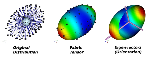
For MIL (mean intercept length), SLD (star length distribution), SVD (star volume dist.), morphological distributions are computed by a “ray field” method (ray field through RVE). The original distribution can be approximated by an ellipsoid, general 2nd or general 4th order tensor.
GST (gradient structure tensor) can be computed from segmented or gray-level images. Beside the required parameters only ‘in’, ‘out’, ‘dtype’, ‘gstpow’, ‘norm’, ‘sort’, ‘grap’, and ‘mod’ are implemented.
In case of MSL (mean surface length) a triangulated surface is used to compute the fabric directly. Beside the required parameters only ‘norm’ and ‘sort’ affects the output.
Eigenvalues and eigenvectors are computed from 2nd order tensors. Graphical output of original and approximated distribution, as well as for eigen vectors is done in Ensight Gold Format. The main information is written in a text file (extension ‘.fab’).
Furthermore, the class mia can be used as library.
Usage
Module
import mia
Command line:
python mia.py ...

  -in       infileName
  -out      outfileName(:mode)
  -dtype    distribType
  -ftype    fabricType
  [-thres]  threshold        [optional]
  [-step]   voxelStep        [optional]
  [-power]  starDirectParam  [optional]
  [-valid]  minIntersectLen  [optional]
  [-code]   code             [optional]
  [-gstpow] gstpow           [optional]
  [-norm]   normalizeType    [optional]
  [-stype]  surfMesherType   [optional]
  [-mod]    outputMode       [optional]
  [-graph]  graphicOutFlag   [optional]
  [-distr]  textOutFlag      [optional]
  [-sort]   sortFlag         [optional]
  [-fout]   fabricOutfile    [optional]
  [-help]                    [optional]
Parameters
- -in
: filename
‘filename’ is a thresholded voxel file. A segmented image (one threshold) with an isotropic resolution is needed. The file is allowed to contain two values: min=0, max=threshold (>0). If the file is not segmented it is necessary to give the option ‘thres’.
- -out
: filename
Text output file where general informations like eigenvectors and eigenvalues are written. 2 possible ways to use it: PARAM: filename -> ‘.fab’ file is written PARAM: filename ‘mod’ option -> Write general information in more compact form (one line) to a file. The “mode” can be “w” (create new file, write header + data) and “a” (append to file, write data).
- -dtype
: type
Distribution type. ‘type’ can be:
‘MIL’: mean intercept length, voxel based
‘SLD’: star length distribution, voxel based
‘SVD’: star volume distribution, voxel based
‘GST’: gradient structure tensor, voxel based
‘MSL’: mean surface length, tria based (Hosseini et.al, Bone 2017)
‘TRI’: mean intercept length, tria based (Laib et.al. Med. Biol. Eng. Comput., 2000)
- -ftype
: type
Type of computed fabric tensor. An approach which is discribed by Zysset 1995 et. al. is used. There, the original distribution computed with the MIL, SLD or SVD method is fitted with a general tensor of second or fourth order. (‘type’=2 or ‘type’=4). Furthermore, an ellipsoid can be used for the fit (‘type’ = 1). For ‘GST’ only ‘type’ = 1 is implemented and ‘MSL’ is not effected by this option.
- -thres
: threshold
Threshold used for the computation of BVTV in case of a given gray-value file. The images is segmented and interally scaled to 0…’threshold’. NOTE: not required for ‘GST’ or in case of a thresholded file.
- -step
: distance
‘distance’ is the number of voxels between individual rays in ray field for the fabric computations. Default = 5; NOTE: not required for ‘GST’, ‘MSL’, ‘TRI’
- -power
: power
Parameter for the computation of the number of star directions on a unit sphere. The number of directions is given by
nDirections = 8*4^'power'
The direction algorithm projects triangles on a unit sphere surface and refines this mesh. The refinement is done by dividing each triangle into four triangles. Default = 2 which gives in sum 128 directions. NOTE: not required for ‘GST’ or ‘MSL’
- -valid
: validLength
Smallest valid intersection length. Intersections are only counted if
isLen > validLength
The intersection length ‘isLen’ is computed from mid-to-mid point of the bone voxels in voxel dimensions (i.e. voxel length = 1).
For example, ‘isLen’ = sqrt(3) means that more then 2 voxel in each direction build a valid intersection. If only one voxel builds the intersections than ‘isLen’=0 and the voxel is not counted if ‘validLength’ = 0. MIL is sensitive to this parameter. Default = 0.0; NOTE: not required for ‘GST’, ‘MSL’, ‘TRI’
- -code
: flag
Type of the used code for the core routines. Possible choices for ‘flag’ are “py2 or “f77”. NOTE: not required for ‘GST’, ‘MSL’, ‘TRI’
- -gstpow
: power
Power coefficient only needed for GST method where the original eigenvalues from the GST evaluation (say l_i) are taken to compute the eigenvalue (m_i) of the fabric M as
m_i = 1.0/l_i**'power'
Default = 0.5
- -norm
: type
Type how the fabric should be normalize. Currently implemented ‘type’ parameters are:
“det” : in that case
m1*m2*m3 = 1(det(M)=1)“rank”/”trace” : in that case
m1+m2+m3 = 3
Default is ‘trace’
- -mod
: mode
The output ‘mode’ can be ‘w’ (create new file, write header + data) and ‘a’ (append to file, write data). Default = ‘w’
- -graph
: flag
Switch on the writing of the original and approximated distributions are written in Ensight Gold Files (‘.case’ and ‘.geo’). ‘flag’ can be “ON” or “OFF”. The results and can be viewed with Paraview Default = “OFF”.
- -distr
: filename
Direction and intercept lengths of original distributions are written to a text file. NOTE: not required for ‘GST’ or ‘MSL’
- -sort
: flag
Switch sorting of eigen values and corresponding eigen vectors. ‘flag’ can be “ON” or “OFF”. Default = “OFF”.
- -fout
: filename
Output quantities to compute the fabric tensors by hand. The parameter specifies the file name.
- -help
: Print usage
Info
File: mia.py
Author: D. H. Pahr
CT Morphometry
Single Run
This scripts analysis the CT based histomorphometry of a bone or similar porous structure based on 3D voxel images. The images have to be binarized with an isotropic resolution. Three destinct gray values (gv) need to be provided:
gv=0 for the mask - the “zero volume” ZV, everything outside the VOI
gv=1 for the background - the marrow, cavities, or pores
gv=2 for the foreground - the bone or solid material
The sum of the volume with gv=1 and gv=2 is the volume of interest (VOI) or total volume TV. Many different histomorphometric parameters can be computed from this definition.
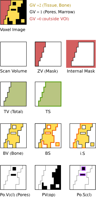
In case of surface and volume data (like bone surface or bone volume) two types of data are analysed:
voxel data showing a zick-zag surface and
smooth triagular surfaces computed from the voxel surfaces.
Smooth surfaces build the interfaces between the compartments and also known as isosurfaces. Directly the interface between the compartments are extracted on a voxel basis. This surface is smoothed where the user can select between two smoothers:
A fast local smoother similar to the idea of marching cubes (default). The advandages are a fast generation und parameter independed surface. However the surfaces is not perfectly smooth as it is usually the case for marching cube based surfaces.
A Taubin’s smoothing algorithm which is acting on the zick-zag surfaces. Although smoother surfaces can be obtained and the Taubin smoothing shows a dependency on the smoothing parameters. Furthermore, it is much slower.
Analysis data are available as text files which can be used in a spreadsheet software or use in Extras - Report Maker to create a PDF.
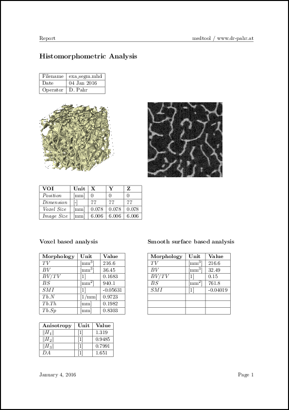
Additionally, graphical output is available for specific data which can be viewed with Paraview. The following picture shows the Tb.Th distribution.
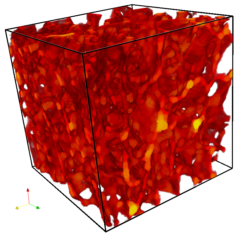
Multi Run
Since medtool version 4.4, this script allows multiple morphological analyses based on ROIs. The model is automatically subdivided into subregions and these regions are individually analyzed. The results are stored on background grid points. If an FEM mesh is provied, then values from the background are interpolated and stored at the centroids of a given FEM mesh.
Compared to the script Material - CT Interpolator, this script is not limited to BVTV and DA and has following additonal features:
all availabe morphometry parameters can analyzed
simplifed usage
multiprocessing is possible
Outputs are available as spreadsheets (CSV) and as graphical output (VTK). Typical Results are shown in the following figure:
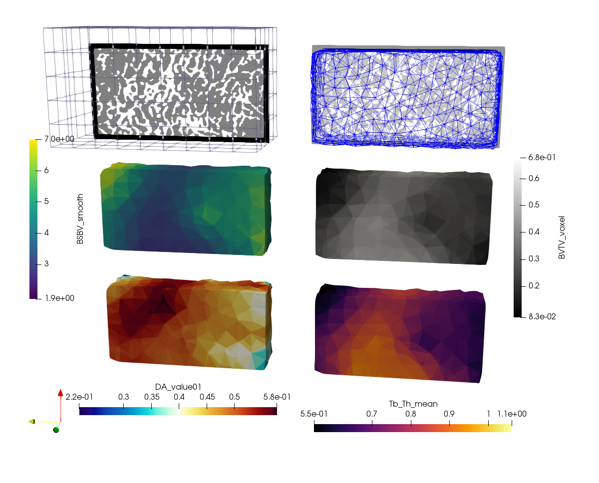
Figure: Top left: input image (0/1/2) with background grid, top right: input image (0/1/2) with FEM mesh, below: typical analysis results interpolated at the FEM mesh.
Usage
Module:
import hma
Command line:
python hma.py ...

   -in     image.mhd
  [-resf   1            ]
  [-smooth 10:0.6307:0.1]
  [-stype  "vxi_m"      ]
  [-norm   "trace"      ]
  [-tbth   ON           ]
  [-tbsp   ON           ]
  [-tbn    ON           ]
  [-smi    ON           ]
  [-da     ON           ]
  [-damsl  ON           ]
  [-datri  ON           ]
  [-bs     ON           ]
  [-is     ON           ]
  [-bv     ON           ]
  [-ts     ON           ]
  [-tv     ON           ]
  [-bvtv   ON           ]
  [-bsbv   ON           ]
  [-bstv   ON           ]
  [-ctth   ON           ]
  [-pos    ON           ]
  [-pov    ON           ]
  [-por    ON           ]
  [-csmi   ON           ]
  [-pon    ON           ]
  [-out    testOut.csv  ]
  [-mrve   7.5          ]
  [-np     4            ]
  [-mmsh   mesh.vtk     ]
  [-mcsv   test.csv     ]
  [-mgra   test.vtk     ]
  [-mod    w            ]
  [-iso    testIso.case ]
  [-oth    testTbth.mhd ]
  [-osp    testTbsp.mhd ]
  [-ofa    testfabr.csv ]
  [-con    ON           ]
  [-gui                 ]
  [-doc                 ]
  [-help                ]
Parameters
- -in
: str
Binary image file name. The file type is recognized by the file extension. The
micmodule (image processor) is used to read the images and all implemented fileformats ofmiccan be used. The images has to show:three gray values (mask=0, background=1, foreground=2) and
isotropic images resolution.
All image processing steps like segmentation, thresholding, cleaning, etc has to be done aforehand.
Optional Parameters
- -resf
: int
Resampling data by factor. The images can be resampled (re-coarsened) by a factor before the analysis. The internal binary image is recoarsened and thresholded by the values 0.5 and 1.5. Note that the change of the image resolution may influence the outcome considerably and should be avoided.
- -smooth
: list
Smooth surface mesh. This filter becomes active if surface or volume data are requested. The implementation follows Taubin’s smoothing algorithm (see, Taubin, Eurographics 2000, Boyd and Mueller 2006). PARAM: niter:lambda:kPB
‘niter’ number of iterations. One iteration means forward (with lambda) and backward smoothing (with mu) smoothing i.e. 2 smoothing steps.
‘lambda’ scaling factor (0<lambda<1)
‘kPB’ pass-band frequency kPB (note kPB=1/lambda+1/mu > 0) => mu
By default a fast smoothed mesh is generated. This option gives more degrees of freedom but is less efficient.
- -stype
: str
Surface mehser type. Implemented types are :
‘vxi_m’: voxel interface extraction followed by a smoothing based on local node moving
‘vxi_mi’: voxel interface extraction followed by a smoothing based on local node moving with one iteration
‘vxi_tb’: voxel interface extraction followed by a smoothing based on a taubin smoothing
The default value is ‘vxi_m’.
- -norm
: str
Type how the fabric in case of DA should be normalize. Currently implemented parameters are:
“det” : in that case
m1*m2*m3 = 1(det(M)=1)“rank”/”trace” : in that case
m1+m2+m3 = 3
Default is ‘trace’
- -bvtv
: str
Bone to total volume BV/TV. BV and TV are used for the computations.
- -bsbv
: str
Bone surface to bone volume BS/BV. BS and BV are used for the computations.
- -bstv
: str
Bone surface to total volume BS/TV. BS and TV are used for the computations.
- -tbth
: str
Trabecular thickness Tb.Th. The method is based on the Hildebrand and Ruesegger method and very similar to the BoneJ implementation. The computation of the thickness is based on following steps:
distance transform (Saito method)
distance transform to distance ridge
distance ridge to local thickness
local thickness cleanup (boundary voxels)
masking with original input image
Maximum, mean, and standard deviation values are available.
- -tbsp
: str
Trabecular spacing Tb.Sp. This is the thickness of the background. It is the ‘tbth’ method applied on an inverted image i.e. background and forground gray values are flipped.
Maximum, mean, and standard deviation values are available.
- -tbn
: str
Trabecular number Tb.N. Computed from:
Tb.N = 1/(Tb.Th+Tb.Sp)
The module checks internall if Tb.Th and Tb.Sp are available and computes them if necessary. Mean values are used for the computations.
- -da
: str
Degree of Anisotropy DA.
The degree of anisotropy is computed based on the mia module using the voxel based Mean Intercept Lenght method (MIL). Additionally eigenvectors and eigenvalues are computed.
- -damsl
: str
Degree of Anisotropy DA based on MSL method (mean surface length) from Hosseini et.al, Bone 2017.
The degree of anisotropy is computed based on a triangulated surface using a dyadic product of the surface normals. Additionally eigenvectors and eigenvalues are computed.
- -datri
: str
Degree of Anisotropy DA based on TRI (Scanco’s method) from Laib et.al. Med. Biol. Eng. Comput., 2000.
The degree of anisotropy is computed based on a triangulated surfaces and calculates the direction distribution by using a scalar product of the area weighted normal vector projected to the direction distribution. Additionally eigenvectors and eigenvalues are computed.
- -bs
: str
Bone surface area BS. This is the surface between the bone and the bone marrow (1/2 grayvalue interface). Smooth and voxel-based surface are computed (see sketch above). The cut surface between bone and the volume-of-interest (VOI), i.e. 0/2 interface, is not included in the calculated value.
- -ts
: str
Total surface area TS. This is the surface area of the volume-of-interest (VOI) i.e. 0/1 + 0/2 interfaces. Smooth and voxel-based surface are computed (see sketch above).
- -is
: str
Intersection surface IS. This is the surface where the bone intersects the VOI i.e. 0/2 grayvalue interfaces. Smooth and voxel-based surface are computed (see sketch above).
- -ts
: str
Total surface area TS. This is the surface area of the volume-of-interest (VOI) i.e. 0/1 + 0/2 interfaces. Smooth and voxel-based surface are computed (see sketch above).
- -bv
: str
Bone volume BV. This is the volume of all foreground voxel (solid objects) within the VOI computed from the smooth isosurface (BV(s)) or voxel images (BV(v)). This is the ‘2’ grayvalue volume.
- -tv
: str
Total volume TV. This is the volume-of-interest (VOI) computed from the smooth isosurface (TV(s)) or voxel images (TV(v)). This is the ‘1+2’ grayvalue volume.
- -ctth
: str
Cortical thickness Ct.Th. The evaluations are using the Tb.Th methode (see ‘tbth’ option). It is provided for confinience.
- -smi
: str Struct Model Index SMI. The calculation of SMI is based on dilation of the 3D voxel model by one voxel thickness. It is computed from:
SMI = 6*((S_2-S_1)*V_1)/S_1^2
where S_1 and V_1 are the bone surface area and volume before dilation, respectively. S_2 is the surface area after dilation. Negative SMI values means the surface area decreases after dilation which may appear in case of closing pores.
- -pon
: str
Pores Number Po.N. Three types of pores are computed:
Po.N(cl): Closed pores in 3D that are fully surrounded on all sides in 3D by bone voxels (GV=2).
Po.N(op): Open pores in 3D that are connected to marrow (GV=1) or the VOI boundary (GV=0) in other words pores with are not closed pores.
Po.N: All pores, open and closed, inside the VOI.
- -pos
: str
Pore Surface Po.S. Three pore surfaces are computed:
Po.S(cl): Closed pore surface in 3D that is fully surrounded on all sides in 3D by bone voxels (GV=2) i.e. the surfaces of the closed pores
Po.S(op): Open pore surface in 3D that is connected to marrow (GV=1) or the VOI boundary (GV=0) i.e. the surface of the open pores.
Po.S: Total pore surface of open and closed pores inside the VOI.
Voxel and smooth surfaces are computed.
- -pov
: str
Pore Volume Po.V.
Po.V(cl): Closed pore volume in 3D that is fully surrounded on all sides in 3D by bone voxels (GV=2) i.e. the volume of the closed pores
Po.V(op): Open pore volume in 3D that is connected to marrow (GV=1) or the VOI boundary (GV=0) i.e. the volume of the open pores.
Po.V: Total pore volume of open and closed pores inside the VOI.
Voxel and smooth surfaces are computed.
- -por
: str
Porosity Po.
Percent of closed porosity within the VOI with respect to the volume of the bone (GV=2) plus the closed pore volume.
- -csmi
: str
Crosssection Moment of Inertia, CSMI.
Average Moments of inertia of the bone crosssectional area (GV=2). Jx, Jy, Jp are calculated from crosssections normal to the z-axis and relative to the respective centers of area.
- -mrve
: int
Size of the reference volume element (RVE) in mm. This option must be active to perform a multiple CT-based morphology analysis.
First, a regular background grid is created (distance is half the RVE size). For each grid point, an RVE of size ‘mrve’ is cropped and analyzed. Results obtained can be output with ‘mcsv’ or ‘mgra’.
If an unstructured mesh (finite element mesh) is passed with the ‘mmsh’ option, then the data from the regular grid are interpolated to the unstructured regular. Interpolated results obtained can be output with ‘mcsv’ or ‘mgra’.
- -np
: int
Number of used CPUs during the run. Must be np>=1. If np=1 the single CPU version is used. The maximum number of given CPUs should not exceed the amount of physicial CPUs on a machine.
- -mmsh
: str
Finite Element Mesh (unstructured grid) file. If this option is active, then the data from the regular grid are interpolated to the unstructured regular. Interpolated results obtained can be output with ‘mcsv’ or ‘mgra’.
- -mcsv
: str CSV Result Output. For example
#NodeId;x;y;z;BVTV_smooth;BVTV_voxel
# min;-1.12;8.48;-1.12;0.0;0.0
# max;23.68;53.12;23.68;1.0;1.0
# mean;11.28;30.8;11.28;0.28892;0.29292
# std;8.47081;14.24651;8.47081;0.19392;0.18894
1;-1.12;8.48;-1.12;0.45403164367878596;0.45072115384615385
2;3.84;8.48;-1.12;0.26324942418717134;0.27100332426715013
3;8.8;8.48;-1.12;0.24431337605344783;0.25163983303518189
4;13.76;8.48;-1.12;0.3508202222156876;0.3542039
...
- -mgra
: str
Graphical Result Output (see Figure above).
- -out
: str
Analysis file name. This is the name of an output file name which includes the analysis data.
- -mod
: str
Write Mode. The output ‘mode’ can be ‘w’ (create new file, write header + data) and ‘a’ (append to existing file, write data). Default = ‘w’
- -oth
: str
Output the trabecular thickness as 3D image file. This file can be viewed with Paraview, Slicer or similar.
- -osp
: str
Output the trabecular spacing as 3D image file. This file can be viewed with Paraview, Slicer or similar.
- -ofa
: str
Output the fabric information form ‘DA’ in a text file.
- -iso
: str
Isosurface file name. This is the name of an output file name which includes the isosurface mesh information. The mesh can be displayed with Paraview or similar.
- -con
: str
Isosurface convergence study. Extracting the isosurface is based on Taubing mesh smoothing. The area change and volume change is computed and displayed. This output helps to find the proper smoothing parameters. See ‘smooth’ option for more details.
- -gui
: Print gui string on stdout.
- -doc
: Print default doc string (__doc__) on stdout..
- -help
: Print help string (extended __doc__) on stdout..
Info
File: hma.py
Author: D. H. Pahr
DXA
The scripts computes a 2D projected image (CTXA) from an 3D QCT image using gray-value projections. Two projection methods are implemented - a pencil (parallel) beam and a cone beam algorithm.
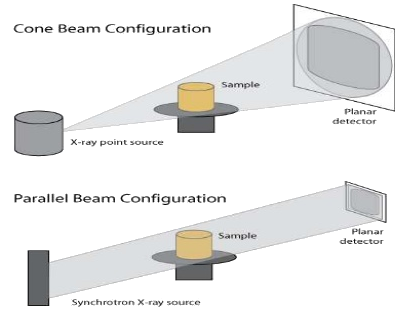
The 3D input gray values are interpreted as BMD in mgHA/cm3 and the output quantity per pixel is BMC in mgHA. The overall BMC is maintained during the computations. An image masks is used to define the global ROI. Additionally, polygons can be given to compute regional quantities like aBMD.
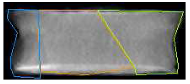
Usage
Command line:
python dxa.py ...

   -inc    testQCT.mhd
   -inm    testMask.mhd
   -dir    1
   -ord    mask_proj
  [-proj   pencil_beam          ]
  [-show   OFF                  ]
  [-deres  0.05;0.05            ]
  [-dedim  1000;1000            ]
  [-dist   800.0;20.0           ]
  [-spsize 0.0;0.0              ]
  [-spoffs 0.0;0.0              ]
  [-refz   1                    ]
  [-din    neck;;5;7;30;10;35;40]
  [-lin    ij1.txt;ij2.txt      ]
  [-width  1                    ]
  [-out    testOut.mhd          ]
  [-mid    test.png             ]
  [-txt    testOut.txt          ]
  [-mod    w                    ]
  [-gui                         ]
  [-doc                         ]
  [-help                        ]
Parameters
- -inc
: filename
Name of the BMD scaled image file (e.g. QCT image). Gray values are interpreted as BMD in (mgHA/cm3)! Available file formats are ‘mhd’, ‘nhdr’, ‘aim’, ‘isq’. Voxel dimensions are assumed to be in ‘mm’!
- -inm
: filename
Name of the mask input file. It has to be scale to 0/1. 0 is outside and 1 is the are where the quantities should summed up i.e. this file defines the global ROI. Available file formats are ‘mhd’, ‘nhdr’, ‘aim’, ‘isq’.
- -dir
: flag
Direction of gray-value projection. ‘flag’ can be 1,-1,2,-2,3 or -3. Positive numbers indicate projections along the axis and negative numbers project the 3D image in the opposite direction.
- -ord
: order
Order of masking/projection operation on the images. ‘order’ can be ‘mask_proj’ or ‘proj_mask’. Note that this gives different outcomes. In case of ‘mask_proj’ the 3D is first masked and projected afterwards.
Optional Parameters
- -proj
: name (str)
Projection method. The 2D projection is computed either by a ‘pencil_beam’ or ‘cone_beam’ projection algorithm. The ‘pencil_beam’ sums up voxel values along the projection direction (1,2, or 3) and is very fast. In contrast ‘cone_beam’ projection uses a fan-based method which needs some kind of interpolation methods. It is computationally much more expensive and rather slow but is able to simulate classical X-rays.
- -show
: flag (str)
Show or check projection. In case of a ‘cone_beam’ projections the overall geometry of the spot, detector, and object size as well as their position can be visualised. The option has implemented ‘OFF’ (no visualization), ‘CHECK’ (show geometry but do not analyse, and ‘SIM’ (analyse and show geometry as well as the projection).
- -deres
: len1;len2 (list[float])
Detector resolution (mm) in case of a ‘cone_beam’ projection.
- -dedim
: nPix1;nPix2 (list[int])
Detector dimension (pixel) in case of a ‘cone_beam’ projection.
- -dist
: SID;OID (list[float])
Source-detector and object-detector distance (mm) in case of a ‘cone_beam’ projection as show in the sketch
_ _
 |                O           <--- focal spot (source)
 |               / \
SID             /   \
 |    _ _      /_____\       <--- object plane
 |     |      /       \
 |    OID    /         \
_|_   _|_   /___________\    <--- detector plane
SID >> 1 and OID = 0 is equivalent to a ‘pencil_beam’ projection. Both parameters influence the magnification of the object.
- -spsize
: len1;len2 (list[float])
Source size (mm) in case of a ‘cone_beam’ projection. A mean filter is used to simulate the unsharpness because of a finite spot size.
  OOOO        <--- finite focal spot
 /    \
/      \
- -spoffs
: len1;len2 (list[float])
Source offset (mm) in case of ‘cone_beam’ projection (see sketch). The default is that the focal spot is place in the center of the projected object
        O
       /.\
      / | \          <--- focal spot (source)
     /  .  \
    /   |   \
   /    xxxxx\        <--- object plane
  /     |-|   \       <--- source offset
 /             \
/_______xxxxxxxx\     <--- detector plane
- -refz
: factor (int)
Refinement factor in z. In case of large voxel size of the object in z-direction, the z-slicing can be increase by a constant factor to increase the accuracy of the project but this comes with an increased computing time. In the following example ‘refz=3’
_______________
_ _ _ _ _ _ _ _
_ _ _ _ _ _ _ _    slize k, 'refz'=3
_______________
- -din
: name1;;i0;j0;i1;j1;…;;;name2;;i0;j0;i1;j1;…
List of voxel ids which define polygons. The ‘name’ indicates the region name. The id list (‘i0;j0;i1;j1;…’) can be obtained with medtools image viewer by picking points with the mouse ( Viewer –> 2D Image Info –> Voxel Id List i;j;… )
- -lin
: filename1;filename2;…
List of files with polygons inside. E.g
file1.txt;file2.txt… One single file contains a list of points ai bi which is used to evaluate quantities inside this area of this polygon. The values are the i,j values of a pixel.These file can be created by hand or an interactive tool like ImageJ (Fiji). Format of a file (space or tab seperated):
41 9
42 82
...
Up to ten files are possible. NOTE: zero gray values are not counted!
The steps to generate text tables containing regions of interest for DXA projection analysis via Fiji/Imagej are:
Start Fiji/Imagej
Open png image with “File”->”Open” (or mhd with “File”->”Import”->”MetaImage”)
Open the ROI manager from the toolbar:
Analyze->Tools->ROI Manager. This allows you to select different regions and to edit them. The ROIs can be saved and opened with this toolSelect the Polgon tool from the toolbar and start drawing
Use the “Add” button in the ROI Manager to add the polygon to the list (ROIs can be modified by clicking on the respective item in the manager list. After modifying the polygon you need to click on the Update button. Saving and opening ROIs is under
More>>.)Each ROI has to be exported to a separate text table containing the corner points: Select the ROI in the manager and export using
File->Save As->XY Coordinates
- -width
: value
Width of the polyline.
- -out
: filename
Output file name where the projection is written as an image. The gray-value per pixel corresponds to BMC in mg.
- -mid
: filename
Output midplanes. If PIL is installed the ROI will be plotted on this image.
- -txt
: filename
Output file name where the computed informations are written in a text file (zero gray values are not counted!
In case if ‘mod’ is not given a typical output looks like:
ROI;   Color;Area (cm2);BMC (g);aBMD (mg/cm2);Volume (cm3);vBMD (mg/cm3)
TOTAL;     -;   9.46187;7.94599;       839.79;     20.8145;      381.752
poly1;orange;   4.01982;3.96436;      986.205
poly2; green;   3.09608;2.65114;       856.29
poly3;  blue;   1.47775;1.01168;      684.608
Otherwise the TOTAL information is written in CSV format:
$ROI;$Area_cm2;$BMC_g;$aBMD_mgcm2;$Volume_cm3;$vBMD_mgcm3
TOTAL;9.46187;7.94599;839.79;20.8145;381.752
- -mod
: str Write Mode. The output ‘mode’ can be ‘w’ (create new file, write header + data) and ‘a’ (append to existing file, write data). Default = ‘w’
- -gui
: Print GUI string on stdout
- -help
: Print usage
Info
File: dxa.py
Author: D. H. Pahr
Grid Data Analyzer
This script reads a series of data files (csv, xlsx format) and creates a Python Pandas data structure called ‘data frame’.
The input data files are generally data distributed in space, e.g. from finite element analyzes or from whole bone analyzes. In this case, an ID (element or node ID) is associated with each data point.
The generate data frame are automatically labelled by a so called index starting with 0. Processing of the data is possible in different ways. Thy can be re-grouped in sub-arrays using the ‘group’ option. By default the regrouping index (order of data entry) can be reset using the ‘index’ option. A new index can be a data column e.g. an element ID or node ID given in the data files.
The generated data frame is automatically marked with a so-called index (starting with 0 after the order of reading in). The processing of the data is possible in different ways. These can be regrouped and analyzed in sub-arrays using the ‘group’ option. By default, the regroup index is the order of data entry. This can be reset with the option ‘Index’. A new index may be a data column from the data files, e.g. an item ID or node ID.
Several Pandas functions can be applied on the regrouped data frame e.g. min, max, mean, std, etc.
A grid data file (mesh+results) can be written (vtk format) to visualize the calculations. For this, the input data must have the same IDs.
Note: It is recommended to read more about Python pandas before using this script (see https://pandas.pydata.org/pandas-docs/stable/10min.html).
Usage
Module:
import gda
Command line:
python gda.py ...

   -inf   testIn.csv
  [-sep   semicolon       ]
  [-eval  VAR3=VAR1+VAR2  ]
  [-index ELEM_ID         ]
  [-group ON              ]
  [-fctn  mean            ]
  [-outi  testIn.csv      ]
  [-outo  testOut.csv     ]
  [-outs  ON              ]
  [-gridm testMesh.inp    ]
  [-dpos  ELEMENT         ]
  [-sdkey VAR1            ]
  [-vdkey U1;U2;U3        ]
  [-gridd testMeshData.vtk]
  [-gui                   ]
  [-doc                   ]
  [-help                  ]
Parameters
- -inf
: filename (str)
Data File Name(s). Python ‘glob.glob’ is used. All the pathnames matching a specified pattern according to the rules used by the Unix shell (
*and?). Examples*data.csv data*.csv data??.csv
A Python pandas data structure called ‘data frame’ is created using the ‘concat’ function. For example, a data frame from three data files may look like
         ELEM_ID   X1   X2   X3  VAR1  VAR2
data1 0        1  1.8  0.0  0.0    15   7.8
      1        3  0.0  2.6  0.0     9  -2.3
      2       10  0.1  0.2  3.4     4   3.5
data2 0        3  0.0  4.6  0.0    19 -12.3
      1        1  3.8  0.0  0.0    25  17.8
      2       10  1.1  2.2  5.4    14  13.5
data3 0        1  6.8  0.0  0.0    35  27.8
      1        3  0.0  7.6  0.0    29 -22.3
      2       10  3.1  4.2  8.4    24  23.5
This is one big array which can be regrouped in sub-arrays using the ‘group’ option. The regrouping index can be reset using the ‘index’ option.
Optional Parameters
- -sep
: optionValue (str)
Delimiter to use. If sep is None, the it will be automatically detect the separator by Python’s builtin sniffer tool, csv.Sniffer.
- -eval
: eq1;eq2;eq3;eq4;eq5;eq6 (str)
Evaluate Equations. Evaluate a string describing operations on DataFrame columns. For example, ‘C = A + B’ will take the column ‘A’, add column ‘B’, and generates a new column ‘C’.
- -index
: indexname (str)
Set index. Set the data frame index (row labels) using an existing columns. The row index (starting at 0) is used as default index. Looking at the abovee example (see ‘inf’ option), the default index is 0,1,2 based on the row numbering. Note in this example that the ‘ELEM_ID’ column does not show the same order. If the computations should not be done by the row ID but by the ‘ELEM_ID’, then the index needs to be reset to ‘ELEM_ID’ by this function.
- -group
: str
Group by index. The data frame can be regrouped by this function. If ‘index’ is not given, then the regrouping is done by the default index (row id starting at 0).
Considering the example from ‘inf’ option, this data frame is treated as one big array. If e.g. the option ‘fctn’ should compute the ‘mean’, then the mean of the whole data frame is calculated. This might be a very expensive computation (takes several minutes!). If ‘fctn’ should be evaluated at all rows with index 0, 1, and 2, then this function needs to be activated. If the ‘fctn’ should be evaluated at the level of ‘ELEM_ID’ columns should be calculated i.e. at 1, 3, and 10, then ‘index’=’ELEM_ID’ needs to be given.
- -fctn
: name (str)
Function Name. If ‘group’ is active, the following functions are implemented
corr()     pairwise correlation of columns, excluding NA/null
           values
cov()      pairwise covariance of columns, excluding NA/null
           values
count()    count non-NA cells for each column or row
describe() generates descriptive statistics that summarize the
           central tendency, dispersion and shape of a datasets
           distribution, excluding NaN values
diff()     first discrete difference of element
min()      minimum of the values in the object
max()      maximum of the values in the object
median()   median of the values for the requested axis
mean()     mean of the values for the requested axis
quantile() values at the given quantile over requested axis,
           a la numpy.percentile
rank()     numerical data ranks (1 through n) along axis
sem()      unbiased standard error of the mean over requested axis
skew()     unbiased skew over requested axis Normalized by N-1
sum()      sum of the values for the requested axis
std()      sample standard deviation over requested axis
var()      unbiased variance over requested axis
nunique()  Series with number of distinct observations over
           requested axis
If ‘group’ is not active additionally following functions are available
abs()       absolute numeric value of each element.
compound()  compound percentage of the values for the requested
            axis
kurt()      unbiased kurtosis over requested axis using Fisher's
            definition of kurtosis (kurtosis of normal == 0.0)
product()   product of the values for the requested axis
round()     round a DataFrame to a variable number of decimal
            places
The output of e.g. the describe() function can be checked if ‘outs’ is active.
- -outi
: filename (str)
Write Input Data Frame. This can be helpful for checks. You should not output too large arrays because all data is written to a single file.
- -outo
: filename (str)
Write Output Data Frame. This array has the size of an input data array and can be processed in a spreadsheet software.
- -outs
: filename (str)
Show Output Data Frame. This can be helpful for checks. You should not output too large arrays because all data are compose prior to output.
- -gridm
: filename (str)
InFile with FEA mesh. The given file is used in case of ‘gridd’ option. It contains an unstructured grid - a mean mesh - which is used to display the results. There are the following requirements on this file is that IDs (NODE or ELEMENT) are exactly the same as the once in the output data frame.
- -dpos
: name (str)
Data Position. This option is needed in case of ‘gridd’ option. It indicates if output variables (IDs) are at the NODE or ELEMENT level.
- -sdkey
: name (str)
Scalar Data Key. This option is needed in case of ‘gridd’ option. The keys are column labels of the output dataframe. Multiple keys an be given e.g. ‘VAR1;VAR2’ and are written as scalar results data.
- -vdkey
: name (list[str])
Vector Data Keys. This option is needed in case of ‘gridd’ option. The keys are column labels of the output dataframe. A single triple - indicating the x, y, z values - need to be given and are written as vector data e.g. ‘X1;X2;X3’
- -gridd
: filename (str)
OutFile with FEA mesh+data. The grid data are taken from the ‘gridm’ options and values from the output dataframe (indicated via ‘sdkey’ or ‘vdkey’ option) are used as results and written to an output vtk file. The result position is know from the ‘dpos’ option. The output file can be viewed e.g. with Paraview.
- -gui
:
Print gui string on stdout.
- -doc
:
Print default doc string (__doc__) on stdout..
- -help
:
Print help string (extended __doc__) on stdout..
Info
File: gda.py
Author: D. H. Pahr
Publish
Report Maker
This script generates a one or multi-page PDF formated report based on Latex. It may include a title, text, figures, tables, and equations which are arranged in a grid layout. The PDF file can viewed with external viewers.
The script is designed to generated fully automatically reports during a parameter run.
Usage
Module:
import rem
Command line:
python rem.py ...

   -pack     title;;title;;;fig1;;fig2;;;eq1;;eq2;;;text1;;-;;;tab1;;tab1
  [-out      report.pdf                                                  ]
  [-pdfview  acroread                                                    ]
  [-mode     begin_part_end                                              ]
  [-pdflatex pdflatex                                                    ]
  [-title    Title                                                       ]
  [-subti    Subtitle                                                    ]
  [-text1    SomeText                                                    ]
  [-text2    SomeText                                                    ]
  [-text3    SomeText                                                    ]
  [-text4    SomeText                                                    ]
  [-text5    SomeText                                                    ]
  [-text6    SomeText                                                    ]
  [-eq1      SomeEquation                                                ]
  [-eq2      SomeEquation                                                ]
  [-eq3      SomeEquation                                                ]
  [-eq4      SomeEquation                                                ]
  [-fig1     fig1.png                                                    ]
  [-fig2     fig2.png                                                    ]
  [-fig3     fig3.png                                                    ]
  [-fig4     fig4.png                                                    ]
  [-fig5     fig5.png                                                    ]
  [-fig6     fig6.png                                                    ]
  [-tab1     a;;1;2;;;b;;3.2                                             ]
  [-tab2     a;;1;2;;;b;;3.2                                             ]
  [-tab3     a;;1;2;;;b;;3.2                                             ]
  [-tab4     a;;1;2;;;b;;3.2                                             ]
  [-head     Report                                                      ]
  [-tesize   11                                                          ]
  [-fisize   0.9                                                         ]
  [-tatyp    2                                                           ]
  [-gui                                                                  ]
  [-doc                                                                  ]
  [-help                                                                 ]
Parameters
- -pack
: column 1;column 2;column 3 (str)
Packer Table. This tables defines a grid layout of the report which means the length and position of the individual elements inside the report. Keywords must be given for the every row and column e.g. title, subti, text1, text2, eq1, eq2, fig1, fig2, tab1, tab2, etc which corresponds to the argument names of the script. Additionally, ‘-’ is interpreted as blank element which means no output is generated.
An element may span over several columns. In this case repeat the keyword. E.g. ‘eq1;;eq1;;text1’ means that ‘eq1’ covers 2/3 ‘text1’ 1/3 of the page width.
Technically a latex document is generated using ‘minipage’ enviroments. The content (text, figure names, etc) is taken from the corresponding option. Therefore, every keyword element in this table must be given.
Optional Parameters
- -out
: filename (str)
Output File Name. This is a PDF file which will be generated by the script. If the option is not active the latex code will be given on the script output area.
- -pdfview
: filename (str)
Pdf Viewer Executable. If this option is activated this pdf viewer will be called to show the generated pdf.
- -mode
: mode (str)
Compose Mode. This option allows to generated a report during a parameter run in medtool. Following options are possible:
‘begin_part_end’: A complete latex file is generated which can be compiled and viewed. This is the preferred option in case of single runs.
‘begin_part’: The beginning of a latex document and the part defined by the ‘pack’ option is generated. More parts can be appended.
‘part’: Only the part defined by the ‘pack’ option is appended to an existing latex file.
‘part_end’: The part defined by the ‘pack’ option and the latex end statement is appended to an existing latex file.
For examples, to generate a report for 4 parameter runs use the following ‘mode’ sequences for the runs:
begin_part - part - part - part_end
This squence can be defined inside a parameter run file.
- -pdflatex
: filename (str)
Pdf Latex Executable. Choose the location of the pdflatex executeable if it is not found automatically.
- -title
: text (str)
Title String. This string is taken as title for the report. A Latex ‘\section*’ statement is used.
- -subti
: text (str)
Sub Title String. This string defines the sub title of the report. A Latex ‘\subsection*’ statement is used.
- -text1
: text (str)
A standard text string. Latex format specifiers can be used. For example use ‘bigskip’ to increase a space, use ‘Large{Some Text}’ to increase the size, etc.
- -text2
: text (str)
A standard text string. Latex format specifiers can be used.
- -text3
: text (str)
A standard text string. Latex format specifiers can be used.
- -text4
: text (str)
A standard text string. Latex format specifiers can be used.
- -text5
: text (str)
A standard text string. Latex format specifiers can be used.
- -text6
: text (str)
A standard text string. Latex format specifiers can be used.
- -eq1
: equation (str)
An equation string. Latex format is used. E.g.
\sigma = E \epsilon
- -eq2
: equation (str)
An equation string. Latex format is used.
- -eq3
: equation (str)
An equation string. Latex format is used.
- -eq4
: equation (str)
An equation string. Latex format is used.
- -eq5
: equation (str)
An equation string. Latex format is used.
- -eq6
: equation (str)
An equation string. Latex format is used.
- -fig1
: filename (str)
Figure file name. ‘png’, ‘pdf’, ‘jpeg’ format is allowed. The size of the figure can be changed with the ‘fisize’ option.
- -fig2
: filename (str)
Figure file name. ‘png’, ‘pdf’, ‘jpeg’ format is allowed.
- -fig3
: filename (str)
Figure file name. ‘png’, ‘pdf’, ‘jpeg’ format is allowed.
- -fig4
: filename (str)
Figure file name. ‘png’, ‘pdf’, ‘jpeg’ format is allowed.
- -fig5
: filename (str)
Figure file name. ‘png’, ‘pdf’, ‘jpeg’ format is allowed.
- -fig6
: filename (str)
Figure file name. ‘png’, ‘pdf’, ‘jpeg’ format is allowed.
- -fig7
: filename (str)
Figure file name. ‘png’, ‘pdf’, ‘jpeg’ format is allowed.
- -fig8
: filename (str)
Figure file name. ‘png’, ‘pdf’, ‘jpeg’ format is allowed.
- -fig9
: filename (str)
Figure file name. ‘png’, ‘pdf’, ‘jpeg’ format is allowed.
- -tab1
: data1;data2;data3 (str)
Table. A table can be given using latex format specifiers e.g. ‘\bf{..}’. The style of the table can be changed with ‘tatyp’ option.
The following format gives a 2x2 table:
a;;1;2;;;b;;3.2
- -tab2
: data1;data2;data3 (str)
Table. A table can be given using latex format specifiers e.g. ‘\bf{..}’. The style of the table can be changed with ‘tatyp’ option.
- -tab3
: data1;data2;data3 (str)
Table. A table can be given using latex format specifiers e.g. ‘\bf{..}’. The style of the table can be changed with ‘tatyp’ option.
- -tab4
: data1;data2;data3 (str)
Table. A table can be given using latex format specifiers e.g. ‘\bf{..}’. The style of the table can be changed with ‘tatyp’ option.
- -tab5
: data1;data2;data3 (str)
Table. A table can be given using latex format specifiers e.g. ‘\bf{..}’. The style of the table can be changed with ‘tatyp’ option.
- -tab6
: data1;data2;data3 (str)
Table. A table can be given using latex format specifiers e.g. ‘\bf{..}’. The style of the table can be changed with ‘tatyp’ option.
- -head
: text (str)
Headline Text. This text is shown in the headline. E.g. it could be the project name, university or company name.
- -tesize
: number (str)
Document Text Size. This is the overall text size and can be 10, 11, or 12 (measured in pt).
- -fisize
: number (float)
Figure Size (0..1). The size of a figure. E.g. 0.9 means the figures spans over 90% of the width of the packing area (known as textwidth in latex).
Also a list can be given. In this case the first value is used for fig1, the second for fig2, etc.
- -tatyp
: type (str)
Table Type. Three basic table style types are possible:
‘1’: a plain table style
‘2’: a classical table without an outer frame
‘3’: a classical table style
- -gui
:
Print gui string on stdout.
- -doc
:
Print default doc string (__doc__) on stdout..
- -help
:
Print help string (extended __doc__) on stdout..
Info
File: rem.py
Author: D. H. Pahr
XY Plotter
The scripts reads an CSV table and creates an XY-Plot based on the column inside the CSV file.
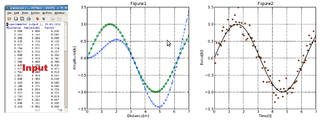
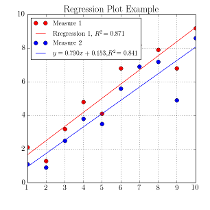
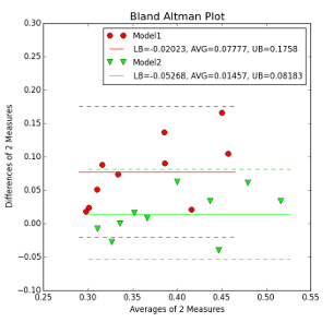
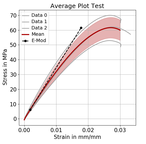
Features are:
Multiple curves in one figure
Polar plots
Error bars
Regression line
Bland-Altman plots
Average Line plots
add user python code
Annotations
Two possibilies are available in case of multiple curves in one figure:
Repeating Arguments: By adding arguments corresponding to the number of curves in figure. The arguments that have to be repeated for each curve in the figure are marked by an ‘*’. Just add another set of arguments, separated by an ‘;’. See ‘infile’ option.
MultiPlot: By loading previous XYPlots and adding curves. (Note that the figure window is created with the first plot of a MultiPlot series. Thus, the first plot settings determine the figure type (normal or polar plot) and its size (-figsize) and axes position (-rect).)
The generate figures can be viewed interactive or written to a file of different foramts like png, eps, pdf, svg, …
Usage
Command line:
python XYPlot.py ...

   -infile*       InfileName
   -cols*         Xdatacolumn:Ydatacolumn
   -sep           Column separator
  [-nheader]*     Number of headerlines                  [optional]
  [-nvarname]*    Index of line with variable name       [optional]
  [-drange]*      Set data range to plot                 [optional]
  [-intervals]*   Set number of pandas df intervals      [optional]
  [-pyplgui]      Show pyplot window                     [optional]
  [-pyadd]        Additional Python commands             [optional]
  Output:
  [-plotfile]     OutfileName                            [optional]
  [-datafile]     OutfileName                            [optional]
  MultiPlot:
  [-mfile]        MultiPlot file                         [optional]
  [-mmod]         MultiPlot mode                         [optional]
  Polar Plot:
  [-polplot]      Polar plot ON or OFF                   [optional]
  [-zero]         Zero degrees position                  [optional]
  Line/Marker Settings:
  [-line]*        Line type and width                    [optional]
  [-lcolor]*      Line color  (r:g:b)                    [optional]
  [-linterp]      Line interpolation method              [optional]
  [-marker]*      Marker type and size. (type:size)      [optional]
  [-mcolor]*      Marker color (r:g:b)                   [optional]
  Errorbars:
  [-xerror]*      Xerrorcolumn code                      [optional]
  [-yerror]*      Yerrorcolumn code                      [optional]
  [-ercap]*       Error bar cap size                     [optional]
  [-errline]*     Error bar line width                   [optional]
  [-errcolor]*    Error bar line color                   [optional]
  [-regline]*     Regression line width                  [optional]
  [-regcolor]*    Regression line color                  [optional]
  [-reglegend]*   Regression legend text                 [optional]
  [-baline]*     Bland Altman line width                 [optional]
  [-bacolor]*    Bland Altman  line color                [optional]
  [-balegend]*   Bland Altman legend text                [optional]
  [-avgline]*     average line width                     [optional]
  [-avgcolor]*    average line color                     [optional]
  [-avglegend]*   average legend text                    [optional]
  [-avgstd]*      average + std dev                      [optional]

  Annotation:
  [-acol]*        Data point annotation column           [optional]
  [-aalign]       Text alignment (horizontal or vertical)[optional]
  [-atable]       Single Annotation with line            [optional]
  Figure and Axes Settings:
  [-figsize]      Figuresize (xsize:ysize).              [optional]
  [-rect]         Axes position in figure (l:b:w:h).     [optional]
  [-xlim]         Axes limits. (xmin:xmax)               [optional]
  [-ylim]         Axes limits. (ymin:ymax)               [optional]
  [-axlabel]      Axes labels. (xlabel:ylabel)           [optional]
  [-legend]*      Legend.                                [optional]
  [-legpos]       Legend position                        [optional]
  [-title]        Figure Title                           [optional]
  [-grid]         Show grid                              [optional]
  [-alpha]        Alpha transparency                     [optional]
  [-xscale]       x-axis scaling (linear or log)         [optional]
  [-yscale]       y-axis scaling (linear or log)         [optional]
  [-fntsztc]      Axes tick labels font size.
  Fontsize:
  [-fntsztc]      Axes tick labels font size.            [optional]
  [-fntszax]      Axes labels font size.                 [optional]
  [-fntsztl]      Title font size.                       [optional]
  [-fntszlg]      Legend font size.                      [optional]
  [-fntszan]      Annotation font size.                  [optional]
  [-tex]          Use TeX ON or OFF                      [optional]
Parameters
- -infile
: filename;…
ASCII-Table file with optional header. Multiple files possible.
- -cols
: x;y;…
Defines x-data:y-data for curve as follows: ‘x’;’y’ whereas ‘x’ is column number of x-data, and ‘y’ the column data for Y. The column numbers start with an ‘c’ Formulas in python syntax possible, e.g.
c3;c4*c5+2
means that x-data is taken from column 3 y-data is computed by formula from columns 4 and 5.
If the name ‘index’ is used (withou column number) the data index (starting with ‘0’) is used.
Furthermore, a variable name (given in option ‘nvarname’) can be used instead of ‘c?’, e.g.
data1;5*data2
Do NOT used ‘$’ in front of variable names i.e. ‘$data1’.
- -sep
: optionValue
Column separator. Any user charactor or the corresponding text like: ‘comma’, ‘colon’, ‘semicolon’, ‘tab’, ‘space’
- -nheader
: count
Number of headerlines which should not be read. default=0
- -nvarname
: count
Index of line with variable name. If this option is active a variable name can given instead of the column number ‘c?’.
For example if the data file looks like
id;data1;data2
1;0.1564;0.9876
2;0.3090;0.9510
an we like to evaluate ‘c1;c2*(c3-1)’ than ‘nvarname=1’ and ‘cols’ reads as
id;data1*(data2-1)
Note that a simple Python string replace function is used i.e. the replace strings have to be unique.
- -drange
: startPos;endPos;…
Plot only a certain part of the data specified by the the given indize ‘startPos’ and ‘endPos’. The first datapoint has index 0 and can be selected by the string ‘start’ (from the beginning). The string ‘end’ means till the end. ‘None’ can be used for None. e.g. ‘10;end’ will plot from the 11th point onward.
- -intervals
: value
Number of pandas invervals. This value is used to create an equidistant pandas data frame between the minimum and maximum x-values of the given data.
The value can be either an integer (=number of created intervals) or a float (=x distance of intervals)
Default: 1000
- -pyplgui
: flag
Open pyplot window after plotting. Possible values are ‘ON’ or ‘OFF’
- -plotfile
: filenname
Output Figure Filename Format. Matplotlib formats are possible: e.g. eps,ps,svg,pdf,png,jpg
- -datafile
: filenname
Output pandas data frame. Possible file formats csv, xlsx
- -pyadd
: filename
After plotting all curves, the python commands in this python file are executed. Can be used to add additional curves, data, annotation to the graph which are not implemented. Figure handle is ‘fig’. Axes handle is ‘ax’. Example:
### original data in dict format
#print(data)
### pandas data frame
#print(pdData)
# calculate E modul from pandas "mean"
ndata = len(pdData["mean"])
skip = int(ndata*0.05)  # skip lower 5%
for i in range(ndata-1):
  if i>skip :
    dx = pdData["x"][i+1] - pdData["x"][i]
    dy = pdData["mean"][i+1] - pdData["mean"][i]
    Ecur = dy/dx
    if i==skip+1 :
      Emod=Ecur
      xmod=pdData["x"][i]
      ymod=pdData["mean"][i]
    else:
      if Ecur > Emod:
        Emod=Ecur
        xmod=pdData["x"][i]
        ymod=pdData["mean"][i]

# add E module to plot manually
legend.append("E-Mod")
xmax = pdData["x"][ndata-1]; ymin = pdData["mean"][0]; ymax = max(pdData["mean"])
pl=ax.plot([xmod,ymax/Emod], [ymod,ymax], linestyle="--", linewidth=2, color="k", marker="o" )
plothandles.append(pl)
- -mfile
: filename
MultiPlot file. Plots may be saved to this file to be opened and appended later. The ‘mmod’ option defines what is done to the file defined here. Example: xyplot.xyplt
- -mmod
: optionValue
MultiPlot mode. Following parameters are implemented
‘w’ The current plot settings are written to the ‘mfile’. Any exising file will be overwritten.
‘a’The current plot settings are appended to the ‘mfile’. All plots of the -mfile AND the current plot are shown.
‘l’The plot settings of the -mfile are loaded. The current settings are disregarded. All plots from the loaded ‘mfile’ are shown.
- -polplot
: optionValue
Polar plot ‘ON’ or ‘OFF’ Then xdata -> angle data (in radiant) Then ydata -> radius data
- -zero
: optionValue
Set zero degree position in polar plot. Options: ‘E’ east (default), ‘W’ west, ‘N’ north, ‘S’ south
- -line
: type;width;….
Line type and width. e.g. ‘-‘;2 (solid line, thickness 2) Line types are: ‘-’, ‘-.’, ‘–’, ‘None’ (no line)
- -lcolor
: r;g;b;…
Line color. RGB values to indicate the color.
- -linterp
: optionValue
Line interpolation method. ‘linear’ (default) or ‘spline’
- -marker
: type;size;…
Marker type and size. e.g. ‘o’;2 (circle, thickness 2) Marker types are:
+ * , . < > D H ^ _ d h o p s v x | None(no markers set).- -mcolor
: r;g;b;…
Marker color. RGB values to indicate the color.
- -xerror
: code;…
Columncode for X-error values. e.g.
c3+c5See ‘cols’ for syntax. ‘None’ for no errorbars.- -yerror
: code;…
Columncode for Y-error values. e.g.
c4*0.1See ‘cols’ for syntax. ‘None’ for no errorbars.- -ercap
: width;…
Error bar cap width. default=4
- -errline
: width;…
Error bar line width. default=1
- -errcolor
: r;g;b;…
Error bar color. RGB values to indicate the color.
- -regline
: width;…
Activates plotting of a regression line. ‘width’ is the line thickness.
- -regcolor
: r;g;b;…
Regression line color. RGB values to indicate the color of the. A solid line is plotted.
- -reglegend
: text1;…
Regression legend text. ‘text’ can be an abitrary string. E.g. “mytext, EQN, R2, SEE”
Following keywords are reserved:
“EQN” is replaced by the regression equations i.e.
y = slope*x + intercept
“R2” is replaced by the squared correlation coefficient i.e. R^2= …
“SEE” is replaced by the standard error of the estimate:
SEE = sqrt( sum(Y-Y')^2 / N-2 ) )
where Y is the actual value and Y’ is the predicted value and N is the number of pairs.
Note: do not use ‘:’ or ‘;’ in this string because these are used as delimiters in case of multi-plots!
- -baline
: width;…
Activates plotting of the three characteristic Bland-Altman lines (-1.96 SD, mean, +1.96 SD, ). ‘width’ is the line thickness of the regression line. The mean is a solid line, the bounds are dashed lines.
Note that the data needs to be evaluated accordingly:
x = (c1+c2)/2 y = (c1-c2)
if c1 contains measurement 1 and c1 contains measurement 2.
- -bacolor
: r;g;b;…
Bland-Altman line colors. RGB values to indicate the color.
- -balegend
: text1;…
Bland-Altman legend text. ‘text’ can be an abitrary string. E.g. “mytext, LB, UB, AVG”
Following keywords are reserved:
“AVG” is the average or mean of the differences
“LB” is the lower bound (SD..standard deviation) i.e.:
LB = mean - 1.96*SD
“UB” is the upper bound (SD..standard deviation) i.e.:
UB = mean + 1.96*SD
Note: do not use ‘:’ or ‘;’ in this string because these are used as delimiters in case of multi-plots!
- -avgline
: width;…
Activates plotting of the average of all given data curves. The max of the minimum x-value and the min of the maxiumum x-value is used.
- -avgcolor
: r;g;b;…
Average line colors. RGB values to indicate the color.
- -avglegend
: text1;…
Average legend text.
- -avglegend
: flag
Switch the plotting of the std dev on or off.
- -acol
: code;…
Annotation column code for annotating each point in the curve. For example: ‘c5_index_c6’ where c? will be replaced by corresponding column data.
- -aalign
: optionValue
Text alignment. ‘horizontal’ (default) or ‘vertical’
- -atable
: xA1;yA1;xB1;yB1;;”Text 1”;;;xA2;yA2;xB2;yB2;;”Text 2”;;;…
Individual Annotations with line between point A and B. Syntax
xA1;yA1;xB1;yB1;;"Text 1";;;xA2;yA2;xB2;yB2;;"Text 2";;;...
- -figsize
: xsize;ysize
Figuresize (xsize;ysize)
- -rect
: left;bottom;width;height
Axes position in figure (left;bottom;width;height). default=0.13;0.13;0.8;0.8
- -xlim
: xmin;xmax
Axes limits. default=automatic
- -ylim
: ymin;ymax
Axes limits. default=automatic
- -axlabel
: xLabel;yLabel
Axes labels.
- -legend
: text1;text2;text3;text4;text5;text6
Legend text string(s) for the curve(s)
- -legpos
: optionValue
- Legend position code 0 to 10: ::
0 best (default) 1 upper right 2 upper left 3 lower left 4 lower right 5 right 6 center left 7 center right 8 lower center 9 upper center 10 center
- -title
: text
Figure Title
- -grid
: flag
Show grid ‘on’ (default) or ‘off’
- -grid
: value
Alpha transparency of markers between 0…1
- -xscale
: optionValue
Scaling of x-axis. ‘linear’ or ‘log’
- -yscale
: optionValue
Scaling of y-axis. ‘linear’ or ‘log’
- -fntsztc
: size
Axes tick labels font size.
- -fntszax
: size
Axes labels font size.
- -fntsztl
: size
Title font size.
- -fntszlg
: size
Legend font size.
- -fntszan
: size
Annotation font size.
- -tex
: optionValue
Use TeX in all Annotations, Labels, Titels, etc in figure. Use
" "if you have blanks in text. e.g.$M^2_i$ in [Nmm]Adding\displaystylewill display the math in math mode. ‘ON’ or ‘OFF’, default=OFF.- -gui
: Print GUI string on stdout
- -help
: Print usage
Info
File: XYPlot.py
Author: A. G. Reisinger, D. H. Pahr
Fabricate
3D Print - FE Modeler
This script generates or reads a segmented voxel image and extracts iso-surfaces from that 3D image. This surface can be modified to create a 3D printing data set.
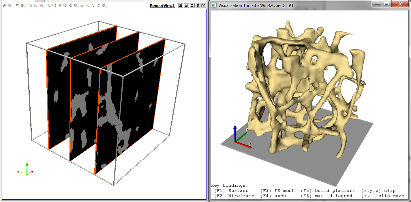
A further feature is that the script can read in a finite element analysis mesh to 1) voxelized the FE models (create a segmented voxel volume) 2) to extract the iso-surface. Solid elements (tetra, hexa, penta, pyra), beams (rods and tapered rods), and shell elements (tria, quad) are supported.
EXAMPLES: mesh and extracted surfaces
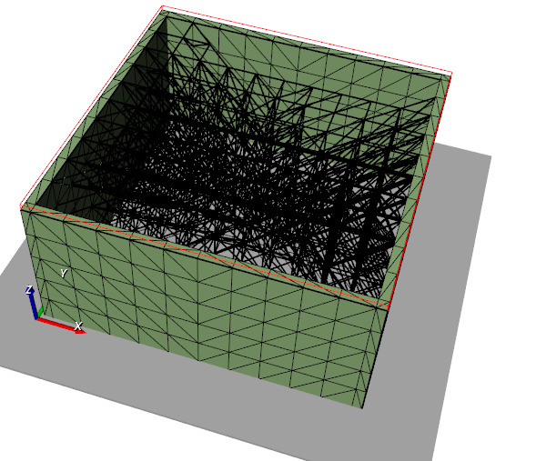
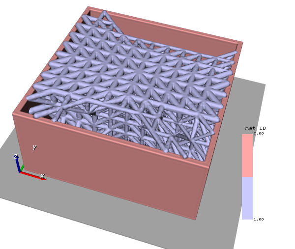
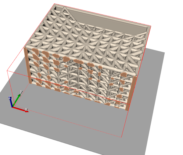
In both cases (direct image or FEA input), iso-surfaces are computed from the segmented images and data files for 3D printing are generated.
EXAMPLES: image (Paraview), extracted surfaces (medtool), sliced model (Cura)
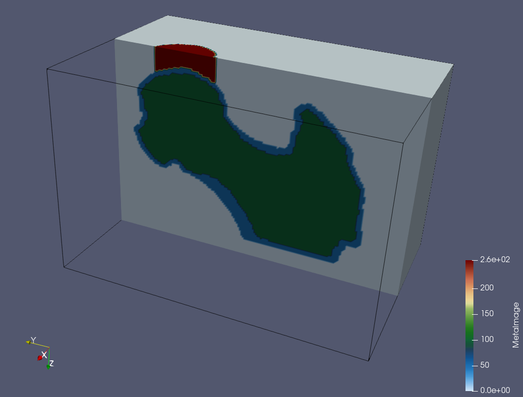
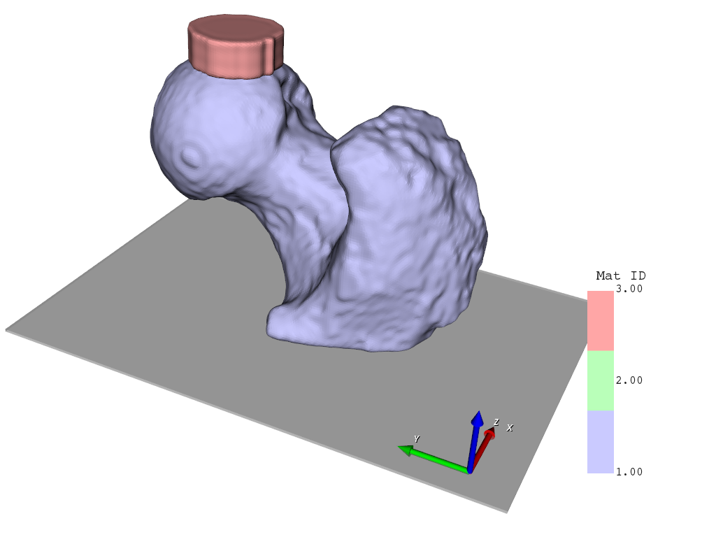
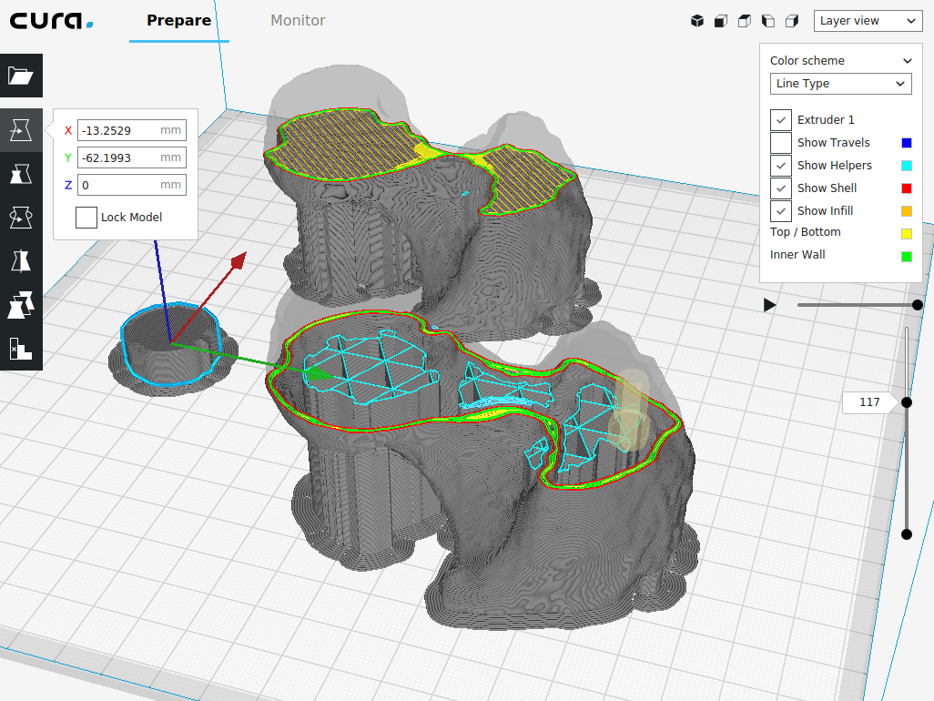
The script has following features :
variable voxel resolutions (FEA only)
single element set extraction (FEA only)
single or multi materials supported
interactive view window
find and flip to strongest print axis
delete unconnected regions in z-direction
change of print axis
fillet option
scale dimension option
voxel model generation (image stacks)
stl surface generation w/wo decimation
screen shots
batch or interactive computing mode
Usage
Module:
import fevox
Command line:
python fevox.py ...

   -fin    test.fem
  [-res    0.1           ]
  [-set    ALL           ]
  [-multi  ON            ]
  [-show   ON            ]
  [-scale  1             ]
  [-fillet 0.6           ]
  [-axis   z             ]
  [-stro   ON            ]
  [-conn   ON            ]
  [-block  100;110;120;0 ]
  [-smooth 20            ]
  [-decim  0.5           ]
  [-size   1024;768      ]
  [-bg     1;1;1         ]
  [-fg     0;0;0         ]
  [-cif    testIn.cam    ]
  [-cof    testOut.cam   ]
  [-outm   test.stl      ]
  [-outi   test.mhd      ]
  [-screen testScreen.png]
  [-mid    testVoxMid.png]
  [-gui                  ]
  [-doc                  ]
  [-help                 ]
Parameters
- -fin
: filename (str)
3D semgmented voxel image or Finite element mesh. Supported file formats containing the segmented voxel image are (isotropic resolutions, smallest gray value have to be zero):
‘.mhd’ : ITK meta image file composed of a header and raw data file.
‘.nhdr’ : NRRD image file composed of a header and raw data file.
‘.isq’ : SCANCO ‘isq’ file format (primary format of SCANCO scanners)
FE mesh formats are :
‘fem’ Optistruct format
‘inp’ Abaqus format
In this case supported elements are :
tetra6, tetra10
penta6, penta15
hexa8, hexa20
pyra5
bar2
tria3
quad4
The material Ids are written for beam or solid sections. In case of quadratic elements only the corner nodes are used. Cylindrical or tapered beams are supported. The end caps of the beams are closed with spheres.
EXAMPLES :
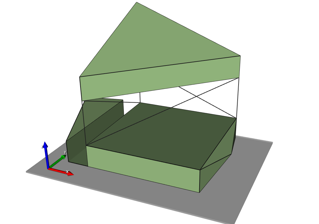
Optional Parameters
- -res
: length (float)
Object resolution in the physical dimension for the voxelization of an FE model. The dimensions is the same as in the FE model e.g. mm or m. Simply spoken the FE elements are filled with isotropic voxels (cubes) as long as the center of gravity of the voxel is inside the element. Higher resolutions lead to higher computations times but finer voxelized and surface meshes.
This option is not required if an image is directly given.
This resolution could be in the range of the 3D printer resolution.
- -set
: set1;set2;set3;set4;set5 (str)
FE set name. If this parameter is activated individual element sets (Abaqus) or property ids (Optistruct) can be read. The default is ‘ALL’ i.e. all elements are used for the voxelization.
- -multi
: flag (str)
This flags activates the multi-material extraction. The material ids are read from the file given by the ‘fin’ option. Internally the gray-level are used starting at 1 for the first element set or property id.
EXAMPLES (single material left, multi material right):
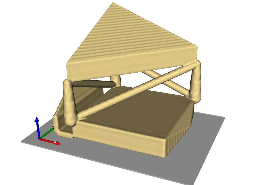
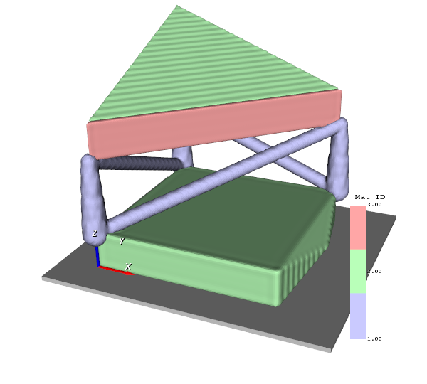
- -show
: flag (str)
Show an interactive render view. This is based on VTK (www.vtk.org) an more details can be found there. The view allows a quick check of the finite element meshes, extracted surfaces, the surface decimation, the print platform (print orientation), and is able to perform clips. All object are set up and toggled ON or OFF interactively.
Mouse bindings are
camera: Button 1 - rotate
        Button 2 - pan
        Button 3 - zoom
        ctrl-Button 1 - spin
actor:  Button 1 - rotate
        Button 2 - pan
        Button 3 - uniform scale
        ctrl-Button 1 - spin
        ctrl-Button 2 - dolly.
Keyboard bindings (upper or lower case) are
F1 - toggle on/off shaded surface (voxelized)
F2 - toggle on/off wireframe
F3 - toggle on/off FE mesh (input)
F4 - toggle on/off print axes
F5 - toggle on/off print platform
F6 - toggle on/off material id legend
x  - toggle on/off x clip
y  - toggle on/off y clip
z  - toggle on/off z clip
+  - move current clip in plus direction
-  - move current clip in minus direction
F7 - print the screen to a file
r - reset camera view
f - fly in / focal point
j - joystick like mouse interactions
t - trackball like mouse interactions
3 - toggle in/out of 3D mode (if supported by renderer)
e - exit
q - exit
- -scale
: factor (float)
This option scales the overall physical dimension of the extracted voxel model and iso-surfaces by the given ‘factor’. 0..1 meas shrinking the models and value >1 means extending the model. Only the voxel model and iso-surfaces are scaled.
- -fillet
: radius (float)
Fillet Radius. Make a fillet on the voxel model. The ‘radius’ gives the size of a spherical kernel. A morphological closing operation is used for this option. This option can not be used if ‘multi’ is active. If surfaces are extracted there is already a small fillet created and this parameter is usually not needed.
EXAMPLES (no fillet left, fillet right):
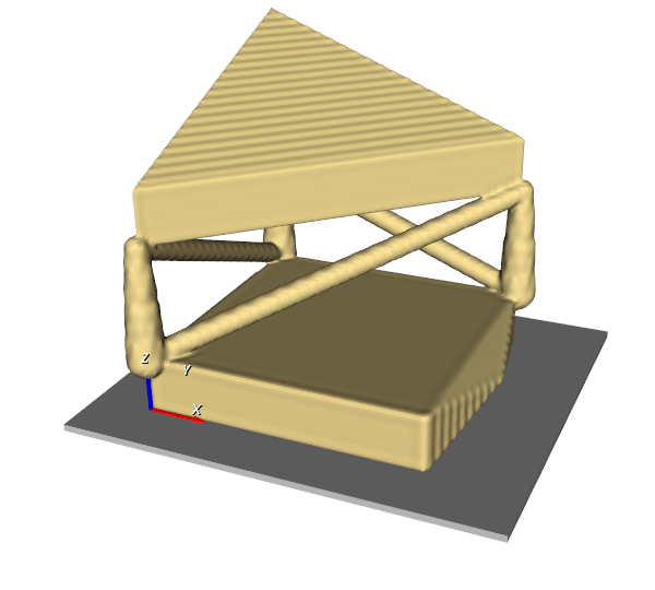
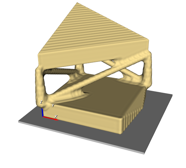
- -axis
: axis (str)
This option specifies the print axis and can be x, y, z. The default axis is the ‘z’ or ‘3’ axis. Changing the axis will flip the voxel model but not the FE model.
The model is flipped along the print axis if ‘-’ is added to the direction.
- -stro
: flag (str)
If this flag is “ON”, the strongest directions is computed based on the cross sectional area and the model is flipped such that z is the strongest direction.
- -conn
: flag (str)
If this flag is activated, the z-directions is checked for unconnected regions slice by slice. Such regions are problematic in case of steriolithography. These regions can be ‘Computed’ or ‘Corrected’.
For example, if the ‘flag’ is ‘Computed’ the image is labelled in the following way
      build platform
==========================
|   111    11         z=0
|   1111  111         z=1
|   11111111     22   z=2
|   1111111    2222   z=3
|   111111111111111   z=4
\/
z-direction
- -block
: nVox1;nVox2;nVox3;grayvalue (list[int])
Place the voxel model inside a bigger block of material. This function can be useful to fit the voxel model exactly to the printer resolution. Parameters are:
‘nVox1’, ‘nVox2’, ‘nVox3’ which are the number of voxels in 1,2,3 direction of the new block
‘newGrayValue’ is the gray-value background of the new block
EXAMPLES :

- -smooth
: nIter (int)
Number of smoothing interations. The extracted marching cubes mesh is automatically smoothed. In case of a decimation a second smoothing step is preformed. A value of ‘0’ means not smoothing. This is critical in combination with decimation. Values bigger than zero perform a volume preserving smoothing of the extracted surface. To see an effect after decimation ‘nIter’>100 is required.
- -decim
: factor (float)
Mesh decimation (0..1). By default an iso-surface mesh is extracted from the voxel image. The surface density depends on the resolution given by the ‘res’ option. This option can be used to decimate the number of triangles. The ‘factor’ is the decimation ratio e.g. 0.9 means that the number of triangles is reduced by 90%. Note that this option can be very time consuming (roughly 10x longer run times).
EXAMPLES (decim=0.0 left, decim=0.8 right):
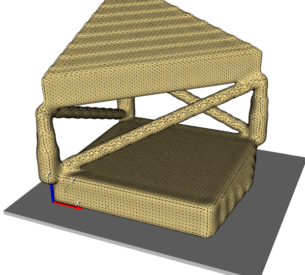
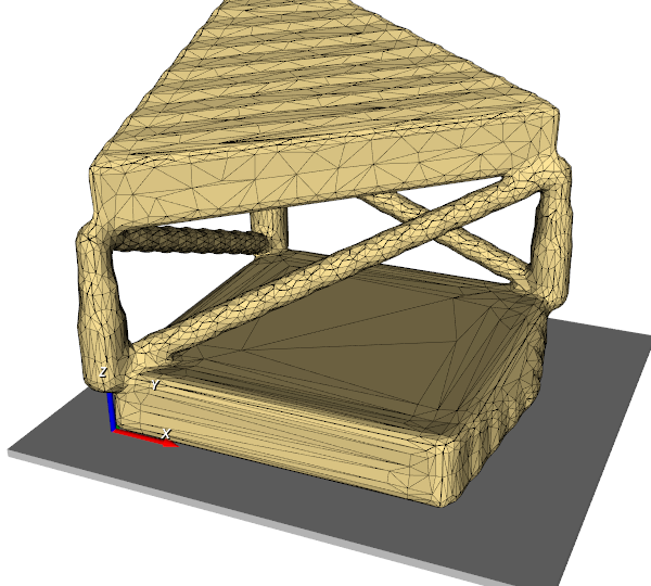
- -size
: sizeX;sizeY (list[int])
Interactive view window size in pixels.
- -bg
: R;G;B (list[float])
Background color of the view window.
- -fg
: R;G;B (list[float])
Foreground color of wire frames and text in view window.
- -cif
: filename (str)
Read camera position form a file. This file can be generated with the ‘cof’ option. Reading a camera position is useful for batch runs.
- -cof
: filename (str)
Write a camera position to a file. This is the final position and will be written after closing the view window with ‘q’ or ‘e’.
- -outm
: filename (str)
Mesh output filename. This is a triangulated file of the extracted iso-surfaces. If ‘obj’ or ‘wrl’ (Vmrl) files are choosen, than the rendering scence is written.
In case of ‘stl’ output, either a single surface or multi surfaces (if ‘multi’ is ‘ON’) are extracted and written. The index for such mulit-surfaces corresponds with the material id show by the VTK interaction window.
- -outi
: filename (str)
Image Output Filename. This is a gray-level image (medical images) which gray-level starting from 1 for each material id.
- -screen
: filename (str)
This option creates a renderer and writes a screenshot from the scene without the need of using the ‘show’ option. It is convenient for batch processing. Available file formats are ‘.png’, ‘.jpg’, ‘.gif’.
Use the ‘cif’ option to control the camera.
EXAMPLE :
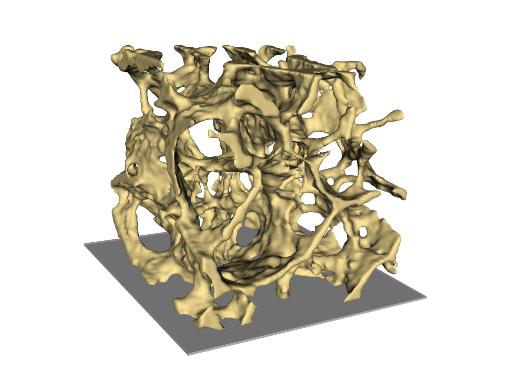
- -scrxyz
: filename (str)
This option creates a renderer and writes three orthogonal views with extensions ‘XM’, ‘YM’, ‘ZM’ which can be viewed with the medtool viewer. In this case the view is updated automatically after a medtool run. Available file formats are ‘.png’, ‘.jpg’, ‘.gif’.
EXAMPLE :
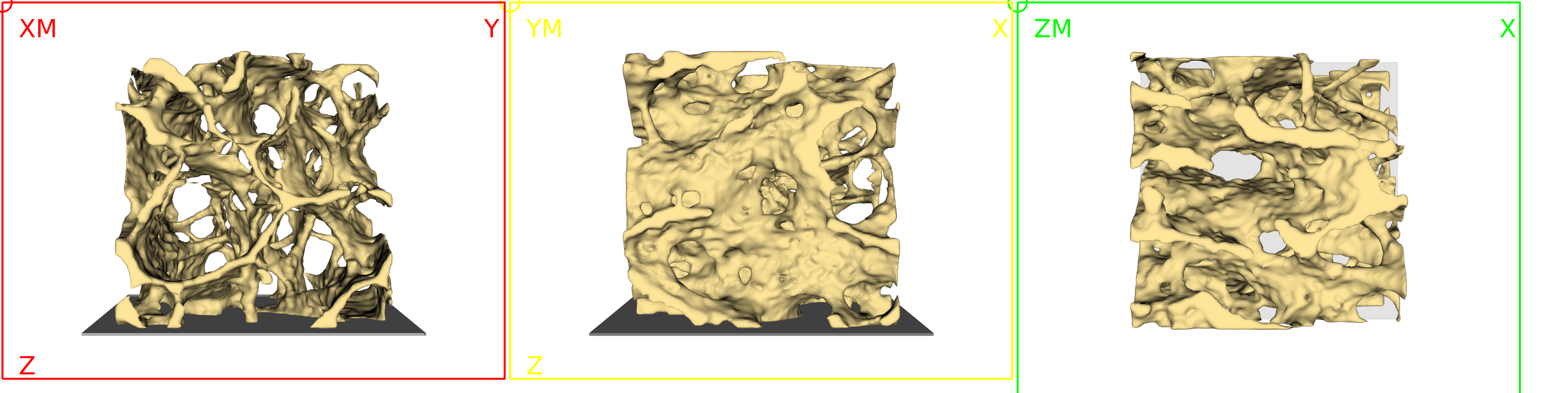
- -mid
: filename (str)
Write mid-plane images of image file (voxel data) in the selected file format. The routine automatically appends “_XM”,”_YM”,”_ZM” at the end of the output file. Compared to the ‘screen’ midplanes from the created images are written which can be checked with medtool.
Available file formats: ‘.png’, ‘.jpg’, ‘.gif’, ‘.tif’, ‘.bmp’, ‘.case’ (Ensight Gold) file format.
- -gui
:
Print gui string on stdout.
- -doc
:
Print default doc string (__doc__) on stdout..
- -help
:
Print help string (extended __doc__) on stdout..
Info
File: fevox.py
Author: D. H. Pahr
Extras
File - Modifier 1
The scripts reads a file with parameters inside ($par1, …) e.g.:
*STEP, PERTURBATION
*STATIC
*BOUNDARY, TYPE=DISPLACEMENT
$topLoad, 1, 2, $value
...
as well as a file with values for these parameters (Excel CSV) e.g.:
$topLoad $value
125      0.94
127      0.86
...
It generates new files where the $ parameters are replace by the
given values in the parameter file e.g.:
File 1                          File2                           File 3
...
*STEP, PERTURBATION             *STEP, PERTURBATION             ...
*STATIC                         *STATIC                         ...
*BOUNDARY, TYPE=DISPLACEMENT    *BOUNDARY, TYPE=DISPLACEMENT    ...
125 , 1, 2, 0.94                127 , 1, 2, 0.86                ...
...                             ...                             ...
Use this script to generate all new files in one shot. Makes not sense inside a parameter run.
Usage
Command line:
python  paf.py ...

  -in     inFileName
  -par    pafName
  -out    outName
Parameters
- -in
: Name of template file with
$par1, … inside. The remaining text in this file will be copied and the$par1will be replaced.- -par
: Parameter file. Example file: :: # comment line -> will be ignored $outfile $par1 $par2 first.txt 1.0 fileA secont.txt 1.5 fileB
- -out
: name of the output file. It can contain variables which are in the parameter file.
- -gui
: Print GUI string on stdout
- -help
: Print usage
Info
File: paf.py
Author: D. H. Pahr
File - Modifier 2
The scripts reads a file with parameters inside ($par1, …) as well as
a file with values for these parameters (e.g. Excel CSV). It generates
new files where the $ parameters are replace by the given values in
the parameter file (CSV).
Use this script to generate the new files during a parameter study at each run.
Usage
Command line:
python  paf.py ...

  -in      inFileName
  -out     outName
  -pal     par1::val1:::par2:val2...
Parameters
- -in
: Name of template file with
$par1, … inside. The remaining text in this file will be copied and the$par1will be replaced.- -out
: name of the output file.
- -pal
: Parameter List: Each entry is composed of on option + value E.g.
file::test.txt:::thres::75The name of the options corresponds to the parameter name (e.g.$file,$thres) and will be replace by the value.- -gui
: Print GUI string on stdout
- -help
: Print usage
Info
File : paf2.py
Author: D. H. Pahr
File - CSV Merger
This scripts creates in the simplest form a new CSV file based on a
source file (including parameter headings e.g. $radius, $filename, $par,
… ) and a list of selected parameter names (e.g. $radius, $filename)
which are extracted. In this simple case, a new CSV file is created which
contains only the selected parameter names.
Additionally, a sink CSV file can be given. In this case the parameters are taken from the source file and used to change the content of the sink file. The following three cases are possible:
The parameter (e.g. ‘$radius’) do not exist in sink file or no sink file is given. Then a column with this parameter is appended on the output file.
The parameter exists in sink file. Then the parameter values in the sink file are replaced by the one from the source file and written to the output.
The parameter exists in the sink file but a new parameter name is given (‘npar’ option). In this case a column with the new parameter name is appended and written to the output.
After the modification, the modified sink content is written into a new file.
The source and sink files need to have following properties:
The first line is a heading line with parameter definitions in it i.e.
$filenam1;$par1;$par2or (without ‘$’)
filenam1;par1;par2
The number of rows must be equal in both files.
Every parameter appears exactly once in the given CSV files. For example, the following file is NOT a valid file because ‘$par2’ appears twice
$filenam1;$par1;$par2;$par2
inf_1.txt;12345;black;gray
inf_2.txt;34890;green;blue
Examples:
If a source file reads as:
$filenam1;$par1;$par3
inf_1.txt;12345;black
inf_2.txt;34890;green
and the parameter ‘$par1’ and ‘$par3’ (‘par’ option) should be modified in the following sink file:
$filenam2;$par1;$par2
inf_1.txt;2.123;black
inf_2.txt;14.53;green
then the result look like:
$filenam2;$par1;$par2;$par3;
inf_1.txt;12345;black;black;
inf_2.txt;34890;green;green;
It should be noted that:
the sink data are not deleted (‘$filenam2’)
but replaced (‘$par1’)
or appended (‘$par3’)
‘$filenam1’ from source is not copied because it is not given in the parameter list (only’$par1’ and ‘$par3’ are given).
The ‘npar’ options allows to change a parameter name during the copy. In this way no replace is done. In the previous example if ‘$par1new’ should be used instead of ‘$par1’ the following result is obtained:
$filenam2;$par1;$par2;$par3;$par1new
inf_1.txt;2.123;black;black;12345
inf_2.txt;14.53;green;green;34890
Note that ‘$par1’ is not changed. Instead ‘$par1new’ is appended.
Usage
Module:
import mcsv
Command line:
python mcsv.py ...

   -source file1.csv
   -sep    semicolon
   -par    par1;par2
  [-sink   file2.csv]
  [-out    test.csv ]
  [-gui             ]
  [-doc             ]
  [-help            ]
Parameters
- -source
: filename (str)
Name of the source input file from which the parameters are read which are specified in the option (‘par’). A comma separated (CSV) text file with delimiter have to be selected.
- -sep
: optionValue (str)
CSV Column Separator. Needed to split the data files. A string like: ‘comma’, ‘colon’, ‘semicolon’, ‘tab’, ‘space’ can be given.
- -par
: parName1;parName2;parName3 (list[str])
Parameter Name List. This option specifies the parameter names which should be read from a source file (‘source’ option) in order to:
create a new file (if ‘sink’ option is not given) or
to replace/append the content of a ‘sink’ file
‘$’ like in a medtool parameter file should not be given they are appended automatically.
For example, if the parameter file contains $radius and $file, the values for this entry are
radius;fileThe string ‘ALL’ reads all parameters from the ‘source’ file.
Optional Parameters
- -sink
: filename (str)
Sink Input File Name. If this file is given the columns indicated by the parameter names (e.g. $radius, …) are replaced or columns are appened if they not exist. The ‘sink’ file is not changed. Only the content is read, modified and written to a new file.
- -npar
: Old Name;New Name (str)
New Parameter Name List. This options allows to change the parameter names from the source in order to avoid replacing columns in the sink with this parameter name. This information is a given as a table in the form ‘par1;;par1new;;;par2;;par2new’ etc.
‘$’ like in a medtool parameter file should not be given they are appended automatically.
- -out
: filename (str)
Output File Name. If this option is given a classical CSV text files is written with separators given by ‘sep’ option.
- -gui
:
Print gui string on stdout.
- -doc
:
Print default doc string (__doc__) on stdout..
- -help
:
Print help string (extended __doc__) on stdout..
Info
File: mcsv.py
Author: D. H. Pahr
User String Runner
The scripts sends a string to the system. This string is taken as it is and executed on the system. It is designed to test quickly external scripts without the need of making a plugin.
Usage
Command line:
python userRun.py ...

      -exe     runString
      -ex1     runString
      -ex2     runString
       ...
Parameters
- -exe
: Run string to be send to the system. Note: use instead of a Single-Quote “ four Single-Apostrophe ‘’’’!
The keywort ‘python_medtool’ can be used to start a script with the python version which is shipped with medtool.
- -exi
: Additional run strings executed one after the other.
- -gui
: Print GUI string on stdout
- -help
: Print usage
Info
File: userRun.py
Author: D. H. Pahr
medtool graphviz
This script creates a graphiz graph from a medtool xml file. It shows shows the input and output options, links the options, colors the nodes according to the script name, i.e. the script node and the input/output nodes of this script show the same color.
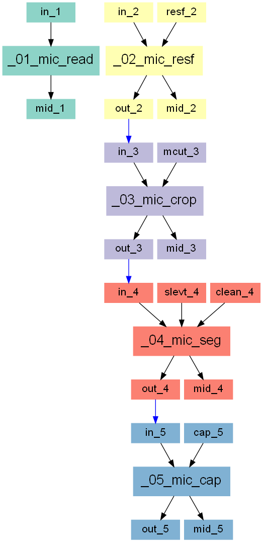
Furthermore, clusters of input/output nodes could be shown.
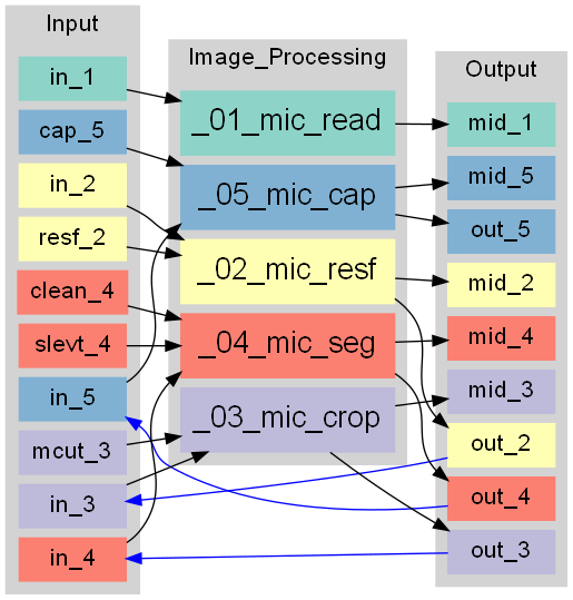
The images and the raw dot file could be written.
Usage
Module:
import mgv
Command line:
python mgv.py ...

   -inf     testIn.xml
  [-out     testOut.png]
  [-simg    OFF        ]
  [-lay     TB         ]
  [-cols    rdylgn     ]
  [-coln    5;1;1      ]
  [-scl     OFF        ]
  [-sli     ON         ]
  [-gui                ]
  [-doc                ]
  [-help               ]
  [-version            ]
  [-author             ]
Parameters
- -inf
: filename (str)
Input File Name. medtool xml file format. The script options are splitted into Input and Output options. Output is recongnized if text ‘Output’ (case insensitive) in description or if type is ‘fileEntryOut’. Everthing else is Input.
Notes for mic scripts:
‘-mid’ option is ignored for linking inputs and outputs
‘-mfil’ option is splitted into the individual options
Optional Parameters
- -out
: filename (str)
Output File Name. Supported file formats are graphics files (png,svg,pd f,gif,jpg) and a dot file.
- -cor
- -simg
: flag (str)
Show Image of Graph or write dot file.
- -lay
: option (str)
Layout of Graph. One of TB (top to bottom), BT, LR (left to right), RL.
- -cols
: option (str)
Color Scheme. Select one of the Brewer schemes from https://graphviz.org/doc/info/colors.html. Note: ‘coln’ is required if ‘cols’ is actived.
- -coln
: Scheme;WhiteStart;WhiteEnd (list[int])
Number of Colors. ‘Scheme’ means number of color scheme colors, ‘WhiteStart’ is the number of how many fontlabels should be ‘white’ at the start, and ‘WhiteEnd’ is the number of how many fontlabels should be ‘white’ at the end. The default fontlabel color is ‘black’.
- -scl
: flag (str)
Show Clusters in Output. medtool sections that begin with “__” are interpreted interpreted as clusters if they are present. This option influences the style significantly.
- -sli
: flag (str)
Show Links. Link input and output in case of “text” values. Numbers are ignored during linking. The arrow from the links are shown in ‘blue’, all other link arrows are ‘black’.
- -gui
:
Print gui string on stdout.
- -doc
:
Print default doc string (__doc__) on stdout..
- -help
:
Print help string (extended __doc__) on stdout..
- -version
:
Print the version on stdout.
- -author
:
Print the author on stdout.
Info
File: mgv.py
Author: D. H. Pahr
Info Text
This script holds a text area with infos. It should be used inside
the medtool GUI with __ (double) or ___ (triple) to get nice
sections which can be made active / inactive with one click.
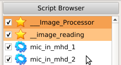
Usage
Command line:
python info.py ...

  -txt      textBLock
Parameters
- -txt
: Text
- -gui
: Print GUI string on stdout
- -help
: Print usage
Info
File: info.py
Author: D. H. Pahr
Archive
These modules are no longer being developed or compiled. It is recommended to switch to new medtool modules with similar functionalities.
Converter - Dicom
This script converts between 3D ITK IMAGE and DICOM formats. It is based on the 2 ITK IO Examples ImageReadImageSeriesWrite.cxx and DicomSeriesReadImageWrite2.cxx Supported file formats:
‘mhd’: VTK meta image file format (‘mhd’ + ‘raw’ file)
‘vtk’: VTK structured grid file format (‘vtk’ file)
‘nhdr’: GIPL format files (‘gipl’ + ‘raw’ file)
- NOTE: DICOM is stored as SHORT i.e. from -32768…+32768. If images are
prived in FLOAT with bigger values they are simply recasted and not scaled! For this task us MIC or ITKCONVERT.
Usage
Command line:
itkDicom ...

  -cdir       ConverstionDirection
  [-snam]     serieName          [optional]
  [-iimg]     inputImage         [optional]
  [-odcm]     outputImage        [optional]
  [-idcm]     inputDir           [optional]
  [-oimg]     outputDir          [optional]
Parameters
- -cdir
: Direction of conversion. Have to be either img->dcm or dcm->img
- -snam
: In case of img->dcm it is an optional name of the series, in case of dcm->img it is the DICOM id if more than one series is in the direction. If not given the default name is ‘image’ or the first series id is chosen
- -iimg
: Input image name, required in case of img->dcm.
- -odcm
: Output directory name, required in case of img->dcm.
- -oimg
: Output image name, required in case of dcm->img.
- -idcm
: Input directory name, required in case of dcm->img.
- -gui
: Print GUI string on stdout
- -help
: Print usage
Info
File: itkDicom.cpp
Author: D. H. Pahr
2D - Marching Cubes
This sripts reads a gray-level voxel model in mhd file format and extracts an isosurface at a given threshold. A modified VTK marching cube algorithm is used for this task which produces sharp boundaries.
Mesh modifications like decimation, smoothing, cleaning, and edge fliping can be performed to obtain high quality meshes meshes.
The obtained 2D meshes can be visualized, used for 3D FE model generations or for 3D printing where a binary STL ouput is available.
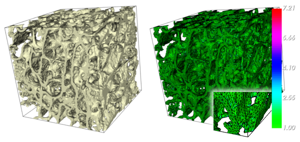
Usage
Command line:
marcher ...

      -in       InFileName
      -out      OutFileName
      -thres    Threshold
      [-coarse] factor                   [optional]
      [-scale]  factor                   [optional]
      [-iter]   iterations               [optional]
      [-decim]  reduction                [optional]
      [-clean]  toleranz                 [optional]
      [-smooth] relaxtion;angle;iter     [optional]
      [-flip]   ratio;angle              [optional]
      [-show]   flag                     [optional]
      [-fg]     R;G;B                    [optional]
      [-bg]     R;G;B                    [optional]
      [-surf]   type                     [optional]
      [-mesh]   flag                     [optional]
      [-size]   sizeX;sizeY              [optional]
      [-screen] filename                 [optional]
Parameters
- -in
: filename
Name of a gray-level file to be used for the iso-surface extraction. Binary images can also be used but do not give but give less smooth initial surface. ‘mhd’ file format is implemented.
- -out
: filename
Name of the iso-surface outputfiles. Follwing formats are implemented:
‘vtk’: Visualization toolkit file format
‘stl’: Binary STL file (preferable for 3D printing)
‘inp’: Abaqus input file format
‘surf’: Netgen mesh file format
- -thres
: value
Threshold for the isosurface extraction. For a 0/1 binary file give 0.5
- -coarse
: factor
Coarsening (resampling) of the mesh before meshing to get a coarser mesh. A linear interpolator is used. A factor of 2 means 8 voxels are resampled to 1 voxel.
Note: High resampling lead to connectivity loss between small structures Default: 1 (no coarsening).
- -scale
: factor
Scale dimensions of the model. Dimensions in x,y,z are are multiplied by this factor Default: 1 (no scaling).
- -decim
: TR;PT;FA;BVD;SP
If this option is active a decimation will be done. The parameters have the following meaning.
- ‘TR’ Target reduction factor for the decimation algorithm.
A value of 0.1 will, for example, try to remove 10% of the triangels. 0.0 means no decimation.
‘PT’ Preserve Topology. The value can be ‘ON’ or ‘OFF’. No split or creation of holes is allowed if ‘ON’.
‘FA’ Feature Angle. Angles between two adjacent triangles is greater this value, are considered as feature edges.
‘BVD’ Boundary vertex deletion. The value can be ‘ON’ or ‘OFF’. If ‘OFF’ the target reduction may not be reached.
- -clean
: number
Relative cleaning tolerance related to the inital voxel size. E.g. a value of 0.3 means that edges smaller than 30% of mean voxel length will be deleted. The value is scaled with ‘coarse’ parameter accordingly.
Note: To big values will cause holes in the mesh! Default: 0.0 (no cleaning).
- -smooth
: relaxtion;angle;iter
Volume preserving Laplacian mesh smoothing. Parameters are relaxation, feature angle, and number of iterations. For more details see VTK manuals. Default: 0.0:0.0:1 (no smoothing)
- -flip
: ratio;angle
Triangle edge flipping to improve the mesh quality. Parameters are maximum allowed edge ratio and feature angle. Default: 1000;0 (nearly no flipping)
- -cif
: filename
File from where to read an active camera position.
- -cof
: filename
File where to store the info of the last active camera.
- -lspot
: x;y;z;intensity
Position and intensity of a spot light.
- -ldiff
: value
Intensity of a diffuse light.
- -show
: flag
Opens a viewer window to show the final result. ‘flag’ can ‘ON’ or ‘OFF’.
- -fg
: R;G;B
Sets the foreground color of the render window. RGB values are ranging from 0..1
- -bg
: R;G;B
Sets the background color of the render window. RGB values are ranging from 0..1
- -surf
: type
Specifies how the 2D surface should be shown. Possibilities for ‘type’ are:
‘MS’ one color smooth shading
‘MF’ one color flat shading
‘Q’ for showing the mesh quality an use as fringe color the mesh quality
Default: ‘MS’
- -mesh
: flag
Switch the mesh lines ‘ON’ or ‘OFF’ Note: for big models rendering with mesh lines takes longer. Default: ‘OFF’
- -size
: sizeX;sizeY
Window sizes of the viewer window (see option ‘show’). Default: 800;800
- -para
: flag
Switch parallel projection ‘ON’ or ‘OFF’. Default: ‘OFF’
- -screen
: filename
Save the render window to a file.
- -gui
: Print GUI string on stdout
- -help
: Print usage
Info
File: marcher.cpp
Author: D. H. Pahr
Stiffness - Error
This script computes the logarithmic stiffness errors for isotropic and orthotropic stiffness tensors versus a given anisotropic tensor and writes the results to an output file. The isotropic tensor is computed by using the closest euclidian distance by Norris, 2006.
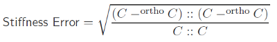
The orthotropic tensor is computed by setting the off-axis terms to 0. Values for the closest isotropic tensor are also written to the output.
Usage
Command line:
python stiffErr.py ...

   -in       infileName
   [-out]    outFilename    (optional)
   [-mod]    outputMode     (optional)
   [-add]    addInfileName  (optional)
   [-sym]    symmetrization (optional)
Parameters
- -in
: filename
Input file: file where stiffness tensor is located. The format of stiffness matrix is:
*STIFFNESS Matrix
11 22 33 23 13 12     ** stress/strain component order
          2           ** symmetrization factor (2..engineering)
****************************************************************
    266.684    84.6788    101.805  -20.32477   15.0725   41.9181
    84.6788    420.372    140.205  -23.7989   -9.33104 -5.306796
    101.805    140.205    616.398  -17.82424  -17.2486   6.92973
  -20.32477   -23.7989  -17.82423   88.9022   -2.20084  -12.6718
    15.0725   -9.33104   -17.2486  -2.20084    61.8393  -2.28074
    41.9181  -5.306796    6.92973  -12.67183  -2.28074   39.7272
- -out
: filename
Output file for analysis results. Depending on the ‘mod’ option a new file will be created or the data will be append to an existing file.
- -mod
: mode
Write mode. Currently following modes are implemented:
‘w’ … write variables and header to outfile (delete old data)
‘a’ … append data to outfile
Default: w
- -add
: filename
Additional input file. File where the stiffness tensor is located from which the orthotropic part should be taken. If this file is not given, the orthotropic part will be taken from the first given stiffness (‘in’ option)
- -sym
: flag
If parameter is “ON” stiffness matrix given by ‘in’ will be artificially symmetrized. This is necessary in the case stiffness tensors computed by PMUBC but has no physical meaning!
- -gui
: Print GUI string on stdout
- -help
: Print usage
Info
File: stiffErr.py
Author: D. H. Pahr
Stiffness - Regression
Script computes the regression parameters for morphology-elasticity relationship based on given orthotropic stiffness tensors, BVTV and eigenvalues.
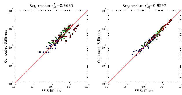
Usage
Command line:
python stiffRegr.py ...

   -in       infileName
   -model    modelName
   [-E0]     fixedE0      (optional)
   [-out]    outfileName  (optional)
   [-mod]    outputMode   (optional)
   [-plot]   plotFileName (optional)
   [-show]   showMode     (optional)
   [-help]                (optional)
Parameters
- -in
: filename
Input file: file where stiffness tensor, BVTV and eigenvalues are located. The format is:
#  E_1   E_2    E_3  G_23  G_13  G_12 nu_23 nu_31 nu_12  BVTV   l1   l2   l3
#[MPa] [MPa]  [MPa] [MPa] [MPa] [MPa]   [1]   [1]   [1]   [1]
129.4  353.6  521.2  86.6  61.2  38.6  0.14  0.13  0.16 0.170 0.73 0.99 1.36
375.8  142.1  730.2  59.7 132.6  43.9  0.07  0.18  0.41 0.210 1.02 0.68 1.42
 13.1   10.9   13.6  17.5   3.9   3.5  0.60  0.09  0.18 0.057 0.87 0.83 1.37
 86.2   77.9  459.0  23.2  37.2  12.7  0.04  0.10  0.20 0.133 1.00 0.68 1.45
392.2  362.3 1392.2 141.4 147.8  67.7  0.12  0.09  0.24 0.283 0.81 0.77 1.59
- -model
: type
Model name. Implemented types are:
‘ortho_opt’ : orthotropic Zysset by optimization and log on stiffness terms
‘ortho_opt_sd’ : orthotropic Zysset by optimization and log on eigenvalues of spectral decomposition
‘iso_opt’ : isotropic Zysset by optimization and log on stiffness terms
‘iso_opt_sd’ : isotropic Zysset by optimizationand log on eigenvalues of spectral decomposition
- -out
: filename
Output file. File where transformed stiffness information will be written.
- -mod
: mode
Write mode. Currently following modes are implemented:
‘w’ … write variables and header to outfile (delete old data)
‘a’ … append data to outfile
Default: w
- -EO
: value
If this ‘value’ is given, a fixed value for the tissue modulus is used during optimization.
- -txt
: filename
Output the results in a text file.
- -plot
: filename
Select a filename to plot the correlation Color code: red…E, green…G, blue…offset terms (nu)
- -show
: flag
Show a correlation plot using matplotlib by using ‘ON’ or ‘OFF’.
- -help
: Print usage
Info
File: stiffRegr.py
Author: D. H. Pahr
Stiffness - Concatenater
Script reads elasticity tensor, applies transformations and outputs CSV files which can be e.g. used in Excel.
Usage
Command line:
python stiffOut.py ...

  -in       filename
  -out      filename
  -var      varid1;varid2;...
  [-mode]   writeMode          (optional)
  [-var]    varid1;varid2;...  (optional)
  [-trafo]  type;par1;par2...  (optional)
  [-ortho]  flag               (optional)
  [-add]    data1;data2;...    (optional)
  [-help]                      (optional)
Parameters
- -in
: filename
Input file. File where stiffness tensor is located. The format of stiffness matrix is:
*STIFFNESS Matrix
11 22 33 23 13 12     ** stress/strain component order
          2           ** symmetrization factor (2..engineering)
****************************************************************
    266.684    84.6788    101.805  -20.32477   15.0725   41.9181
    84.6788    420.372    140.205  -23.7989   -9.33104 -5.306796
    101.805    140.205    616.398  -17.82424  -17.2486   6.92973
  -20.32477   -23.7989  -17.82423   88.9022  -2.20084  -12.67183
    15.0725   -9.33104   -17.2486  -2.20084   61.8393  -2.28074
    41.9181  -5.306796    6.92973  12.67183  -2.28074   39.7272
- -out
: filename
Output file. File where transformed stiffness information will be written. A typical output looks like:
#InputFileName;$E_1;$E_2;$E_3;$G_23;$G_13;$G_12;$nu_23;$nu_13;...
cyl1.out;2.23e+11;2.22e+11;2.22e+11;8.6e+10;8.71e+10;8.70e+10;...
cyl2.out;1.04e+11;1.02e+11;1.01e+11;3.9e+10;4.06e+10;4.04e+10;...
cyl3.out;5.93e+10;5.65e+10;5.51e+10;2.1e+10;2.31e+10;2.29e+10;...
...
- -var
: varid1;varid2;…
Variable id’s which should be written. Currently implemented:
E_1, E_2, E_3… Young’s moduliG_13, G_23, G_12… shear modulinu_13, nu_23, nu_12, nu_31, nu_32, nu_21… Poisson ratio’sK… Bulk modulus (=``1/9*sum(Eij)`` with i,j=1-3)
The order of the out is the order of the given Variable id’s.
- -mod
: mode
Write mode. Currently following modes are implemented:
‘w’ … write variables and header to outfile (deletes old data)
‘a’ … append data to outfile
Default: w
- -trafo
: type;par1;par2;…
Transformations applied on the stiffness matrix. Currently implemented:
‘type’=”rotmax2, rotate such that E_1=Emax, E_2=Emid, E_3=Emin
‘type’=”rot”. Additional parameters for this options are axiA;axiB;axiC;ang1;ang2;ang3
where:
axiA;axiB;axiC = Rotation order around axis. For example 3;1;2 means first the model is rotated around 3-axis, second around 1 axis and third around 2 axis
ang1;ang2;ang3 = Rotation angles in Deg around 1,2,3 axis. That means ang1 will be applied in the previous examples as second rotation.
Note: if the angles are taken from sop.py (Stiffness Optimizer) the model have to be rotated such that rotation order = 1;2;3 and rotation angle = x;y;z (from sop)
- -ortho
: flag
If ‘flag’=”ON” only orthotropic part of stiffness is used. IF “OFF” the original matrix will be used.
- -add
: data1;data2;…
Additional data which should also put on the output and are simply treated as strings. This can be useful if the output is used in a spreadsheet software.
- -help
: Print usage
Info
File: stiffOut.py
Author: D. H. Pahr
Stiffness - Optimizer
This programs rotates a given anisotropic elasticity tensor such that that best orthotropic fit is reached. This is done by optimization and is based on the work of Van Rietbergen et.al, J Biomech, 1996.
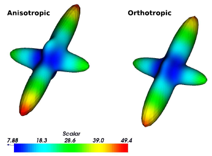
It writes an echo of the computed stiffness, roational angles. Furthermore it put out an xy file containing the values of the minimization functions and writes the orthotropic and anisotropic stiffness tensor as well as the axis of orthotropy in Ensight Gold ‘.case’ format for Paraview.
Usage
Command line:
python sop.py ...

  -stf     stiffnessInputFileName
  -out     outputFileName
  [-fkt]   funktionType            [optional]
  [-alg]   algorithmType           [optional]
  [-start] angle1:angle2:angle3    [optional]
  [-xy]    filename:rotAxis        [optional]
Parameters
- -stf
: filename
Name of the file where the stiffness matrix is located. A special format is needed, where the order of the stress/strain components and the symmetrization faktor (=2 for engineering type) is supported. Example:
*STIFFNESS Matrix
11 22 33 23 13 12     ** stress/strain component order
          2           ** symmetrization factor (2..engineering)
********************************************************************
    266.684    84.6788    101.805  -20.32477   15.0725   41.9181
    84.6788    420.372    140.205  -23.7989   -9.33104 -5.306796
    101.805    140.205    616.398  -17.82424  -17.2486   6.92973
  -20.32477   -23.7989  -17.82423   88.9022   -2.20084  -12.67183
    15.0725   -9.33104   -17.2486  -2.20084    61.8393  -2.28074
    41.9181  -5.306796    6.92973  -12.67183  -2.28074   39.7272
- -out
: filename
Name of the output file where the analysis echo will be written.
- -fkt
: type
Type of optimization (error) funktion which will be used. Possible options for ‘type’ are ‘offAxisError’, ‘strainError’, ‘stressError’
- -alg
: type
Applied optimization algorithm. Options for ‘type’ are ‘fmin’ or ‘fminBFGS’. If the BFGS algorithm does not find an solution within an allowed number of iterations the optimizer switches auto- matically to the ‘fmin’ algorithm.
- -start
: angle1;angle2;angle3
Estimation of start rotation angle e.g. 0;45;13. in deg. This option is useful if the algorithm finds a local minima.
- -xy
: filename;axis
Name of a xy plot file which should contained the values of the optimization functions (error) over an angle of 0…180 deg. Furthermore the rotational axis has to be given. e.g. file.txt;3 The angles for the other axis are taken from the optimization.
- -help
: Print usage
Info
File: sop.py
Author: D. H. Pahr
Stiffness - Visualizer
Script reads elasticity tensor and writes a ‘.case’ file (ensight gold format), which can be read and displayed by Paraview.
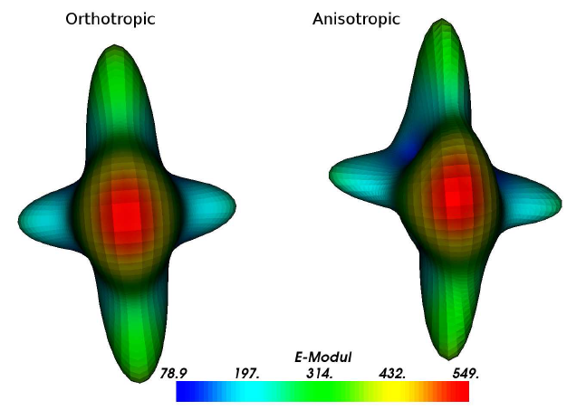
Usage
Command line:
python mia-ext.py ...

     -in       InfileName
     -out      OutfileName
   [-lout]     limitedOutput    (optional)
   [-help]                      (optional)
Parameters
- -in
: filename
Input file. File where stiffness tensor is located. The format of the given stiffness matrix is:
*STIFFNESS Matrix
11 22 33 23 13 12     ** stress/strain component order
          2           ** symmetrization factor (2..engineering)
********************************************************************
    266.684    84.6788    101.805  -20.32477   15.0725   41.9181
    84.6788    420.372    140.205  -23.7989   -9.33104 -5.306796
    101.805    140.205    616.398  -17.82424  -17.2486   6.92973
  -20.32477   -23.7989  -17.82423   88.9022  -2.20084  -12.67183
    15.0725   -9.33104   -17.2486  -2.20084   61.8393  -2.28074
    41.9181  -5.306796    6.92973  12.67183  -2.28074   39.7272
- -out
: filename
Output file. File where stiffness information will be written.
- -lout
: flag
Output flag of engineering/bulk modulus distributions Options for ‘flag’ are :
‘E’ … Distribution and scalar data is the E-modulus
‘K’ … Distribution and scalar data is uniaxial bulk modulus K
‘EK’ … Distribution is E and scalar data is K
- -help
: Print usage
Info
File: mia-Stiff.py
Author: D. H. Pahr
Stiffness - Modeller
The scripts computes the iso- and orthotropic stiffness tensor for a given fabric-elasticity model type based on BV/TV and fabric. It writes a text file of the stiffness matrix which can be used in ‘Stiffness’ - ‘visualizer’ to generate a 2D surface of the tensor.
Usage
Command line:
python stiffModel.py ...

  [-iso]    E0;nu0;k                       [optional]
  [-ortho]  E0;nu0;G0;k;l                  [optional]
  -bvtv     density
  [-mi]     m1;m2;m3                       [optional]
  [-ev1]    e1x;e1y;e1z                    [optional]
  [-ev2]    e2x;e2y;e2z                    [optional]
  [-ev3]    e3x;e3y;e3z                    [optional]
  [-out]    filename                       [optional]
Parameters
- -iso
: E0;nu0;k
Isotropic density-elasticity model type. ‘E0’ is the Young’s modulus, ‘nu0’ the Poisson’s ratio, and ‘k’ is the power coeffizient of the power law. The E-modulus is computed from
E = E0 * (BV/TV)^k
Note: Either ‘ortho’ or ‘iso’ option has to be given.
- -ortho
: E0;nu0;G0;k;l
Orthotropic fabric-elasticity model type by Zysset. ‘E0’ is the Young’s modulus, ‘nu0’ the Poisson’s ratio, ‘G0’ the shear modulus, ‘k’ is the power coeffizient of the power law, and ‘l’ is the power coefficient for the fabric.
Note: Either ‘ortho’ or ‘iso’ option has to be given.
- -bvtv
: density
‘density’ is the bone volume over total volume (BV/TV). The range is 0…1.
- -mi
: m1;m2;m3
Fabric eigenvalues used in the ORTHOtropic model. The order will be computed automatically.
- -ev1
: e1x;e1y;e1z
First fabric eigenvector needed for ORTHOtropic model. It has to be the corresponding vector for m1.
- -ev2
: e2x;e2y;e2z
Second fabric eigenvector needed for ORTHOtropic model. It has to be the corresponding vector for m2.
- -ev3
: e3x;e3y;e3z
Third fabric eigenvector needed for ORTHOtropic model. It has to be the corresponding vector for m3.
- -out
: filename
Name of output file where stiffness info will be written. The stifness matrix is written as ASCII text. This file can be used in ‘Stiffness’ - ‘visualizer’ to generate a file which can be viewed in Paraview.
- -gui
: Print GUI string on stdout
- -help
: Print usage
Info
File: stiffModel.py
Author: D. H. Pahr