Examples
This section contains simple examples medtool to introduce new users to the software and show the functionality of medtool for advanced users.
In addition to these examples, there are also a variety of Youtube videos (https://www.youtube.com/channel/UCMYES6oxqwsoUufl5-ONoHg) that give a first impression of medtool.
The examples are included in the medtool distribution and are found in the install directory. It is recommended to copy the examples to a location with read / write permissions (e.g. to the home folder).
When first opening a medtool ‘.xml’ in the corresponding example folder, a warning appears that the working directory is not found.
The easiest way is to confirm the suggested working directory (it is the folder of the example), or a new working directory can be selected with Run Settings - Working Directory. All new generated files have the prefix “exa” to be able to delete them after running an example easily.
Here are some guidelines how to work through the examples:
- New users
All new users should first go through the section.
- FEA Users
Start with the sections Image Processing followed by the example Image to FEA. Further examples are Image Calibration and Image to Smooth Mesh (CGAL) followed by the FEA Material Mapping example.
- Users from Anthropology
Start with the sections Image Processing followed by the example CT Bone Morphometry.
After understanding the basic idea of *medtool*, one is ready to work through more complex examples.
Image Processing
Note
User Level: Simple
Image processing is the first step after receiving 3D images from a CT or MRI scanner. medtool includes many image processing capabilities. In this example a high-resolution CT scan of a trabecular bone biopsy is used.
For this first example, it is recommended to open the medtool database file (‘.xml * file) from the folder example. If not set automatically, change the working director to the directory where you extracted this example (using Run Settings - Working directory). After this initial set up, no file paths need to be provided.
Since medtool 4.4 user levels are introduced. This examples opens with the user level “Simple”. As a result, only a limited number of tool bars and script options are visible.
Following working steps are demonstrated inside this example:
read and check a medical 3D image
re-size the image by a factor of 2
crop out a cubical region of interest (ROI) with 4 mm side length
segment the image with an automatic threshold and clean it
add an other solid material at the top and bottom of the ROI
The following scripts will be created:
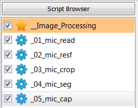
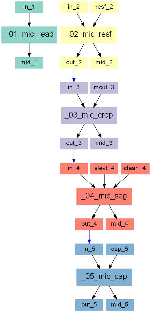
The entire workflow looks like this:
Step 1
Create a new script from the menu Image - Processor (simply click on the Image menu)
and denote it as _01_mic_read. ‘_01’ means this is the first processing step i.e. or
the first script (Note: the underline is necessary because a script name is not allowed to
start with a number 0-9).
‘mic’ is a shortcut of the script (‘mic.py’), ‘read’ means we are simply reading a content,
in this case a CT image.
Select a file under (-in) option by clicking on the folder symbol and selecting the
file ‘spongyBone5.mhd’. Activate the mid-plane output (-mid) by clicking on the check box and
insert as output name ‘exa.png’.
After clicking Run ... (Menu Run - Run Active or short cut on the tool bar on the left side)
the scripts executes. The GUI looks like:
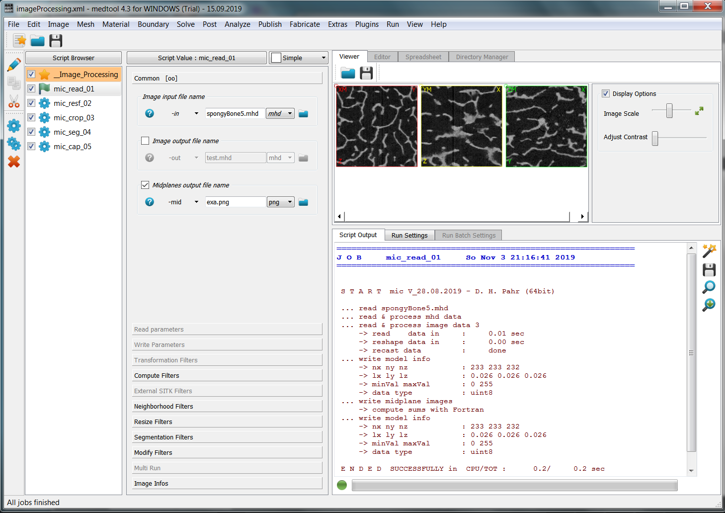
and more details are visible in the Script Output area:
S T A R T  mic V_28.08.2019 - D. H. Pahr (64bit)

... read spongyBone5.mhd
... read & process mhd data
... read & process image data 3
    -> read    data in     :     0.00 sec
    -> reshape data in     :     0.00 sec
    -> recast data         :     done
... write model info
    -> nx ny nz            : 233 233 232
    -> lx ly lz            : 0.026 0.026 0.026
    -> minVal maxVal       : 0 255
    -> data type           : uint8
... write midplane images
... write model info
    -> nx ny nz            : 233 233 232
    -> lx ly lz            : 0.026 0.026 0.026
    -> minVal maxVal       : 0 255
    -> data type           : uint8
    -> compute sums with Fortran

E N D E D  SUCCESSFULLY in  CPU/TOT :      0.1/     0.1 sec
medtool informs the user about every processing step. In this case which files are read and, furthermore, some basic informations like the number of voxels (nx, ny, nz), the sizes (lx, ly, lz, here in mm), and the gray-value range. In a second step, the mid-planes are written and again the model info is displayed. Since no processing has been done yet, the input and output information regarding the image (voxel model) is the same.
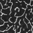
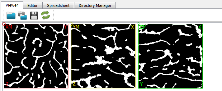
After running the script, we open the midplane with View - Viewer. The mid-planes and are shown in the right upper Viewer area. The mid-planes can be scaled and the contrast can be adjusted. Switching from user level ‘Simple’ to ‘Standard’ or ‘Expert’ allows more viewer options.
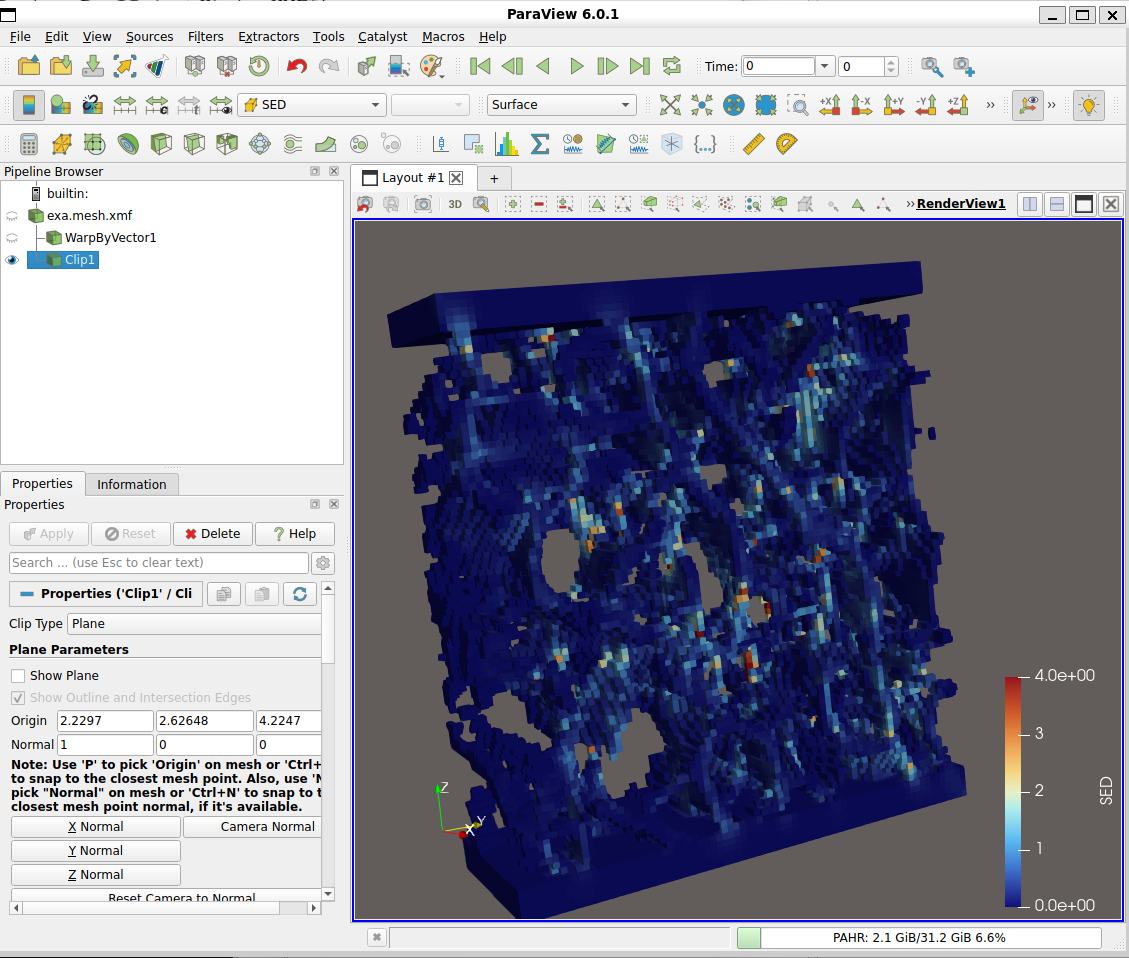
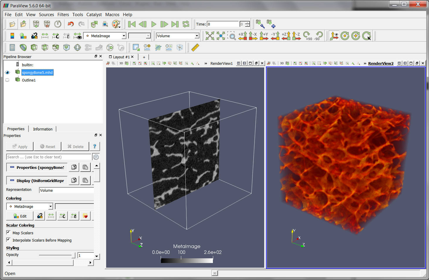
The content of the image file (‘.mhd’) can be also checked with other tools, for example, with ParaView:
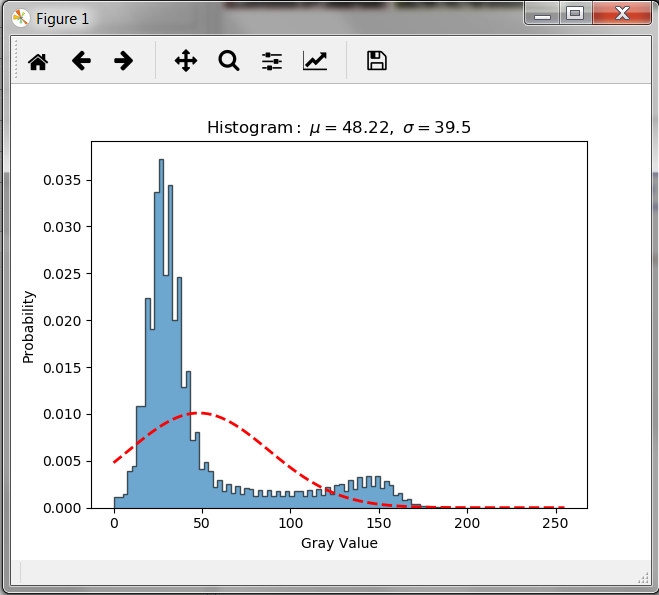
A histogram of the image data can be viewed by selecting the Image Info tab of this script, activating the ‘shist’ option and setting a value of ‘0’. After re-running the following window pops up:
Step 2
Open a new instance of Image - Processor and call it to _02_mic_resf.
Alternatively copy the previous script instance. Here, ‘02’ means the second step,
‘mic’ is a shortcut for the script, and ‘resf’ indicates the activated option (resize by factor).
The image is re-sized in this step by a constant factor of 2 using the Resize
Filters tab and selecting the option -resf. In this way we avoid errors from partial volume
effects because exactly 8 voxels are are condensed into one coarse voxel.
More re-coarsening options are available by changing the user level.
Note
If you like to get more help on the individual options, activate it by clicking on the help sign near the option. Alternatively, you can look at this help.
The new image is written to an image file (‘exa_mic_resf.mhd’) and also the mid-planes (‘exa.png’) are written.
If the same mid-plane output file name is used as under step 1 an automatic update of the images inside the Viewer is generated.
The re-coarsening is visible also in the Script Output Area :
... write model info
    -> nx ny nz            : 116 116 116
    -> lx ly lz            : 0.052 0.052 0.052
    -> minVal maxVal       : 0 188.75
    -> data type           : None
    -> compute sums with Fortran
The number of voxels and the image resolution changes. Note that one voxel layer is removed in x an y direction (originally 233 voxels) by this function.
Step 3
Open a new Image - Processor instance and call it _03_mic_crop. The input
image -in is the output image of the previous step (‘exa_mic_resf.mhd’) and the
new ouput image is called ‘exa_mic_resf.mhd’ (-out option).
In order to get approximately 4 mm side length we need around 77 voxels in x, y, and z.
The image is cropped with the Resize Filter -mcut for example (crop from the middle).
Graphically we get:

and numerically:
... write model info
    -> nx ny nz            : 77 77 77
    -> lx ly lz            : 0.052 0.052 0.052
    -> minVal maxVal       : 0 179
    -> internal data type  : float32
The change of the size is visible but the resolution is unchanged compared to step 2.
Step 4
In this step a binary image is obtained by using the Segmentation Filters panel.
-slevt is an automatic segmentation (single level thresholding) propsed by
Ridler and Calward 1978.

To clean the image (remove flying voxels) switch on Modify Filters -clean option. This options looks
for the largest connected piece of material inside the voxel model.
Step 5
In the final step we put end caps at the model ends (Modify Filters -cap) in 3-direction. This is usually done to mimic embedding of such a sample during an experimental test in case of simulation models.
The final result looks like:
Further comments
To re-run everything, check all script instances and click Run - Run Checked or the Icon near the Script Browser.
Don’t forget to save the database and to clean up the working directory.
Image Calibration
Note
User Level: Expert
Usually, CT scanners are calibrated with respect to water. The obtained CT numbers are called Hounsfield units (HU). Typically HU is “-1000” for air and “0” for water across the whole CT source energy spectrum. Since the linear x-ray attenuation depends on many factors, such HU values need to be further calibrated for each biological tissue of interest. Such corrections are based on CT measurements of liquid or solid bone equivalent materials with known bone mineral density (BMD). A calibration relationship between HUs and BMD has to be established to correct the CT images and to obtain a quantitative CT image (QCT). The following example shows how such a calibration is done within medtool.
The images calibration consists of the following steps
explore the image
label the phantom region of interests (ROIs),
establish a calibration relationship (linear, quadratic, …),
use this to recompute the HUs to BMD equivalent CT numbers.
The entire workflow looks like this:
Please work through the example Image Processing before you start with this one.
Step 1
In a first step the image and corresponding data are explored.
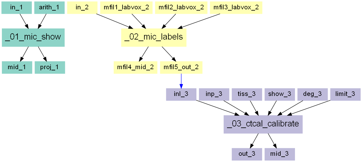
Create an Image - Processor script and name it _01_mic_show.
Next, perform the following steps:
Select from the example folder the file
ctImage.mhdfor-inoption.Activate the
-midoption and change the file name toexa.pngRun the script (single run).
Open the midplanes with medtool’s Viewer and load the file
exa-XM.png.
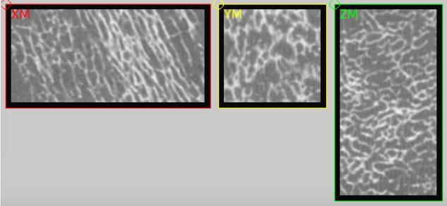
The GUI shows in the Viewer area:
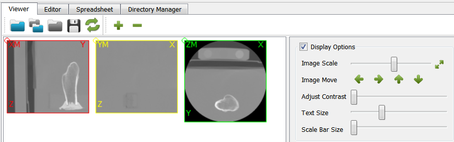
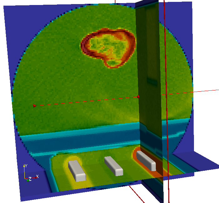
There is a bone and a phantom (circles in ZM slice) inside the image. Inside the info area we see that:
the gray values ranges from -2048..1622 (typical for CT images)
the spacing of the voxels is anisotropic and between 1.0 .. 1.404 (for this example dataset the image was recoarsened by a factor of 4 in all directions)
there is an offset of the origin which depends on the CT scanner
The phantom chambers are hard to see. Thus, we improve the contrast by change the gray value range of the image. This can be done if we:
Check the gray values by clicking on the chambers (circles) inside the Viewer.
At the panel next to the image (2D Image Info (mouse pick) area) shows the value inside the *Gray Value field. Values of around 168 (left), 10 (middle), and 297 (right) are obtained for the three chambers.
Now we change the images by selecting the
-arithCompute Filters and modify the image accordingly: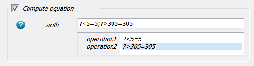
The image is cut-off between 5 .. 305 (our interested values are between 10 and 297). Note: This step is only done for visualization!
Run the script and the midplane is automatically updated:
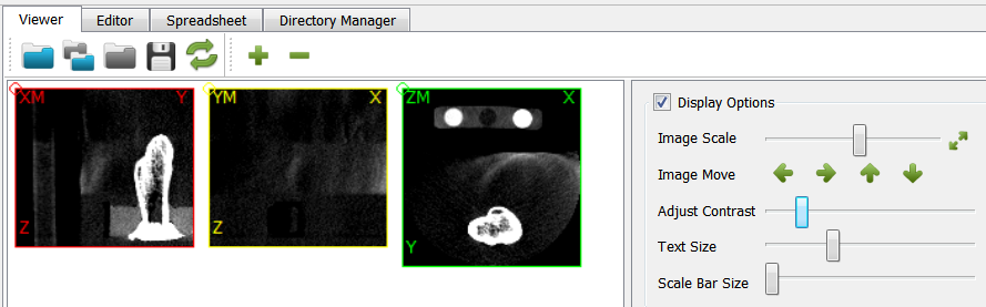
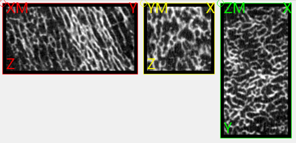
More contrast is visible but it is hard to see what kind of bone it is. Thus let us:
Activate also the
-proj(projected midplane) option and give a file nameexa.pngRun the script.
Open the midplane the Viewer and load one of the file
exa-XP.png(Note thePin the filename).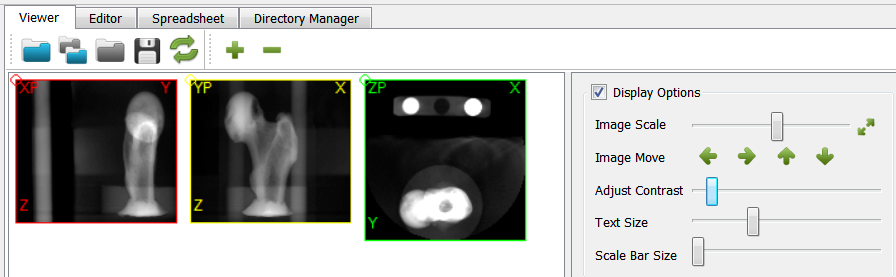
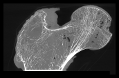
The midplanes are know like X-ray images (projections) and we see that the bone is a human femur.
Finally, the generated files are explored using a file explorer from your operating system. The working folder looks like :
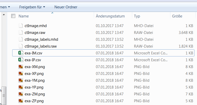
Six png files are generated. Three midplanes ::
exa-XM.png
exa-YM.png
exa-ZM.png
and three projected midplanes:
exa-XP.png
exa-YP.png
exa-ZP.png
Furthermore two csv files are generated:
exa-IM.csv
exa-IP.csv
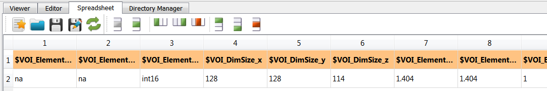
which contain informations about the images. They can be opened and explored with medtool’s Speadsheet editor:
Step 2
Different calibration procedures are possible: in-scan calibration where simultaneously a
phantom is scanned with the subject or asynchronous calibration where patient and phantom
scans are separated. In both cases the regions of interest with known BMD have to be
labelled. Taking the image ctImage.mhd, one needs to label the phantom chambers
(circular rods). For medtool’s calibration script, the regions have to show following
gray-values:
0(outside),1(first calibration chamber),2(second calibration chamber),etc.
The calibration chambers are called ROIs (regions of interest). In medtool, ROIs can be selected with the Viewer and extracted or cropped with the Image - Processor. Therefore,
ROIs have to be selected:
Generate and open a midplane - e.g.
exa-XM.pngfrom above.Look into medtool’s Viewer manual and learn how to select a ROI. The resulting selections of the first chamber looks like:
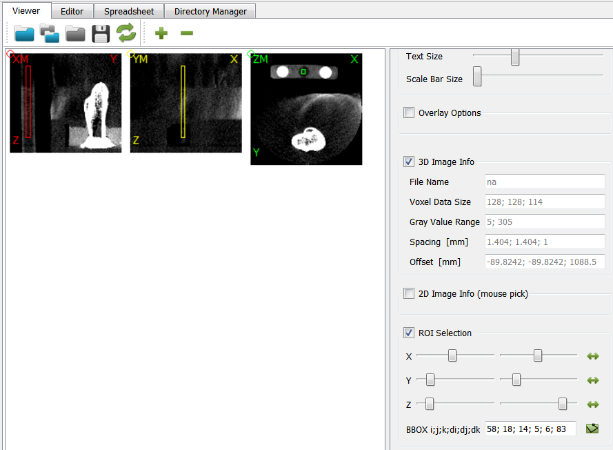
Note that the Viewer’s ROI Selection panel shows inside the BBOX field the bounding box of a ROI in voxel dimensions
59; 18; 14; 5; 6; 83This information can be used to mask or label the image.
Labelled mask of the scan chambers are generated by the following procedure:
Create a new Image Processor script
_02_mic_labels.Select the an image (
ctImage.mhd.) which has the phantom inside using the-inoption.The needed filter which generates the label or mask is the
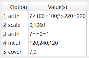
-labvoxfilter inside the Compute Panel. Read the help of this filter to understand the individual options. It needs 8 parameters - 2 gray values for the background and the label itself as well as 6 entries for the BBOX which can be taken from above. The options including the entries looks like: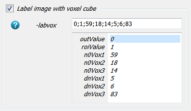
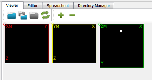
and the resulting image is a simple 0/1 image where the background has a value of 0 and the ROI region has a value of 1:
This procedure needs to be redone three time for each calibration chamber. Therefore, a Multi Run (-mfil) is used and the preveously used
-labvoxfilter is switched off. The ROI selection (step 1 from above) and the labelling is repeated. The resulting entry reads as: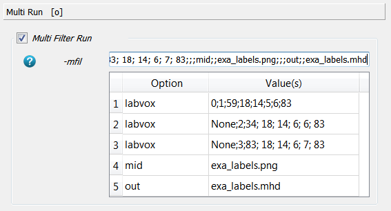
Note that in the second and third
labvoxscript the background (outValue) is set toNonewhich means the background from the input image is taken. Furthermore, the gray value for the two other chambers is 2 and 3, respectively. Finally, after running the script a labelled image is obtained and written to the output: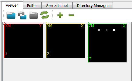
The three chambers are visible. Check this file with Paraview to see if the selections is done correctly, e.g.:
Alternatively, the labelling can be done with a software tools like Fiji (https://fiji.sc/) by using the segmentation editor but also other interactive tools can be used. The resulting image with Fiji looks like :
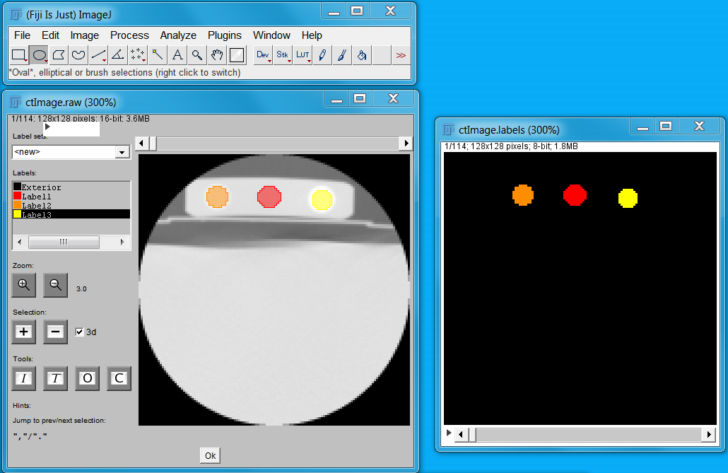
Howto labelling with Fiji’s segmentation editor:
Open Fiji and load the gray-level file (File - Open - select ‘mhd’ File) e.g. ‘ctImage.mhd’
Open the segmentation editor Plugins - Segmentations - Segmentation Editor).
Inside the editor, rename ‘Interior’ to ‘Label1’ by right click on the ‘Interior’ label.
Select the ‘Oval’ tool from the toolbox (top left, next to rectangle). Draw a circle on the first image of the stack. Move to the end of the stack with the slider and draw a second circle.
Next we interpolate between both circles by clicking the I bottom (under Tools). Afterwards we add this to the active label (‘Label1’) and click ‘+’ buttom (under Selection). The ‘3D’ check box should be checked. Note that a new image stack denoted ‘ctImage.labels’ is created and the segmentation is shown in the corresponding color.
For a new label, we right click on ‘Label1’ and click ‘Add Label’. Right click again on the new label and change the color.
Repeat previous steps and create three labels.
Close the segmentation editor.
Finally select the ‘ctImage.labels’ stack in Fiji, click File - Save as - MHA/MHD, and select a file name e.g. ‘ctImage_labels.mhd’. It is important that you also write ‘.mhd’ otherwise an ‘.mha’ file is written. Avoid a ‘.’ in the file name.
This image is also in the example folder and called ctImage_labels.mhd.
Step 3
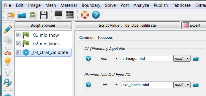
Coming back to medtool, open a medtool, create a new Image - Calibrator instance, and call it ctcal_calibrate.
Go to the -inp option and select the file ‘ctImage.mhd’ from your example folder. This file contains the phantom and the image. It is fine if it only contains the phantom:
Go to the -inl and select the file ‘exa_labels.mhd’ was generated above and contains the ROI labels. It has to have the same shape as the file ctImage.mhd. The GUI should like:
The third required input are the know tissue densities for each label. Choose the default options:
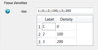
This means that the label 0 is a ROI with 0 mgHA/ccm, label 1 is a ROI with 100 mgHA/ccm, and label 2 has 200 mgHA/ccm. These arbitrary label numbers have to be the same as those used in the file ‘ctImage_labels.mhd’.
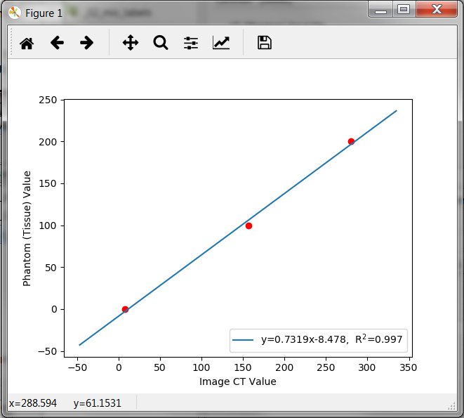
Switch the -show option on to see the calibration result. A window pops up showing the calibration relationship:
Step 4
Let us refine our image calibration procedure. Some important aspects are:
In case of asynchronous calibration an additional input file which should be calibrated can be given with the
-incoption.The
-degoption inside the Calibration Options panel allows the selections of higher order polynomials as calibration relationship.The
-limitoption in the same panel gives the possibility to cut-off values coming either from fat (negative values) or from image artefacts (values beyond reasonable BMD values). This cut-off is also shown with-showoption :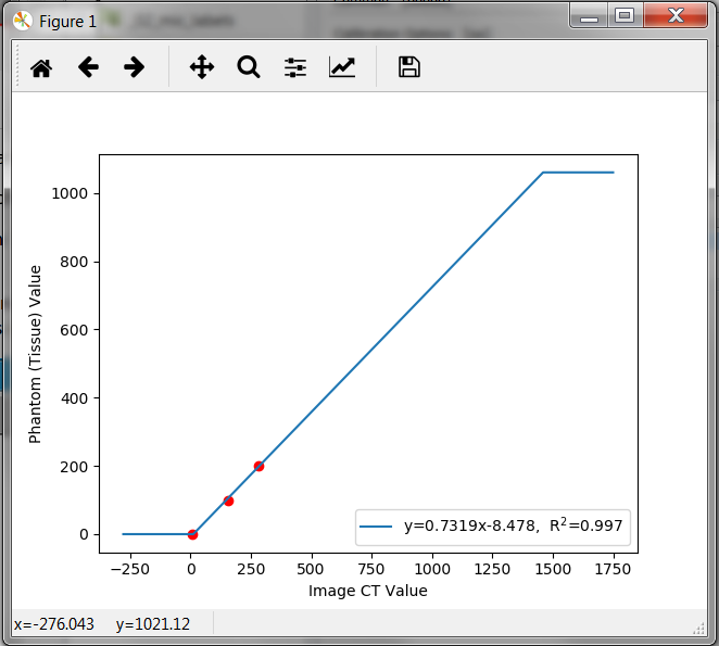
In order to output the resulting image, select
-outoption and give a file name (e.g. ‘exa_ctcal.mhd’) to create a calibrated output image i.e. a quantitative CT (QCT) image.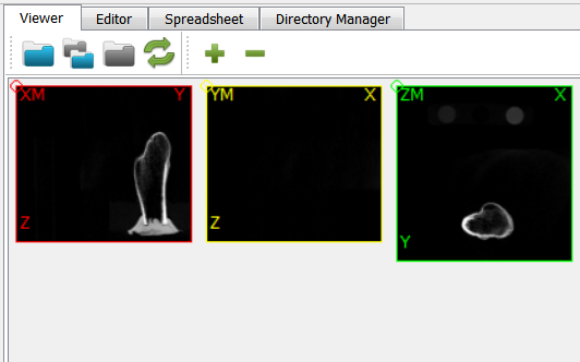
Note the cut-off of the image at the limits. This image is BMD-scaled and can be used FEA simulations.
The Output Options panel allows to write the calibration results to CSV files which can be further as in parameter runs.
#outputfile;label_id;phantom_gv;image_gv;label_id;phantom_gv;image_gv;label_id;phantom_gv;image_gv;
exa_ctcal.mhd;1;0;7.66886;2;100;153.338;3;200;282.249;
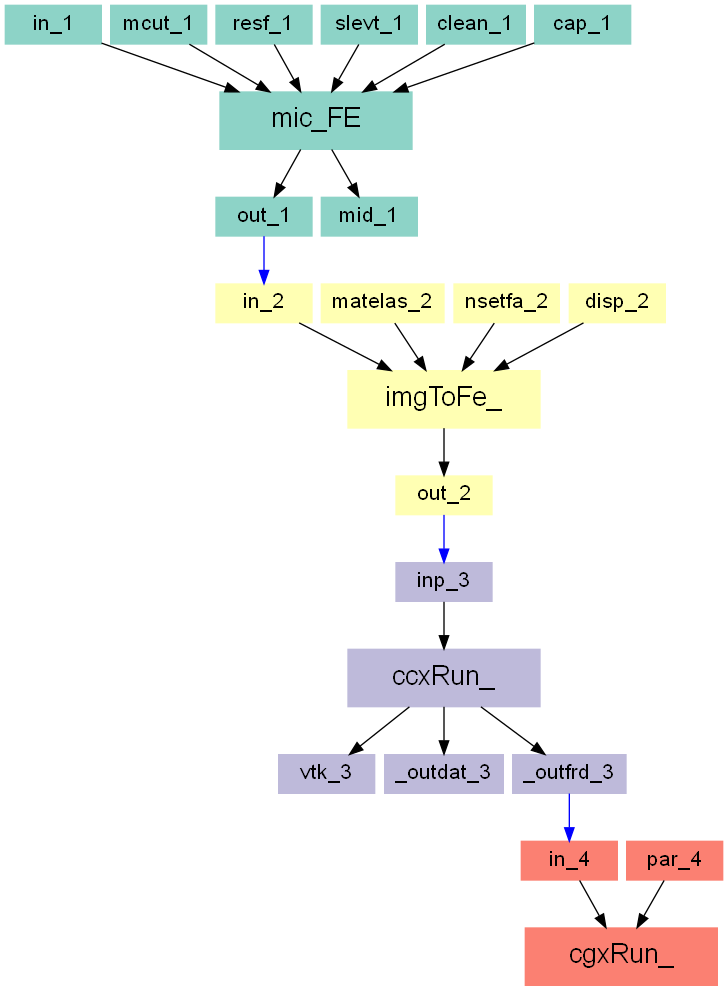
Image to FEA
Note
User Level: Simple
This example demonstrates a direct conversion of a 3D image data file into a voxel based Finite Element model, shows how to run the simulation with Calculix, and how to post-processing the results with Calculix or Paraview.
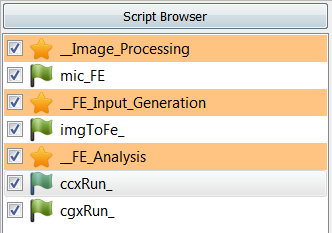
The Image - Processor, Image - FEA Converter, Solve - Calculix, and Post - Calculix scripts are used within this example. Four steps are done:
create a segmented image with end plates
generate an FEA model input deck
solving the model with Calculix ccx
post-processing the model with Calculix cgx and Paraview
The script browser has the following look for this example:
The entire workflow looks like this:
Recommendation: Work through the example Image Processing before you start with this one.
Step 1
This step covers the image processing. A spongy bone file (spongyBone5.mhd)
is loaded and the mid-planes are written to the disk (exa_mid.png). The content of the file
is check wiht the Viewer before the -out option is selected. The XM mid-plane are shown below:

This image is processed by following steps (this is a demo, select reasonable values for real world examples):
cropping the image Resize Filters option
-cut(150 voxels)
resizing the image Resize Filters option
-resf(factor 3)
segment the image Segmentation Filters option
-slevt(default value).
clean the image Modify Filters option
-clean(FAST)
attach a voxel layer to the image Modify Filters option
-cap(one layer in 3 direction, gray-value 255)
Finally the image is exported as exa.mhd using the -out option.
Step 2
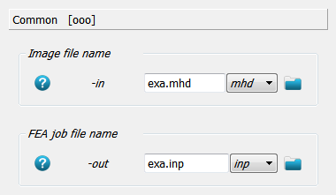
This labelled image is converted to an FEA input deck using Image - Converter FEA - Abaqus, Calculix. First, the input image and output FEA input deck are selected.
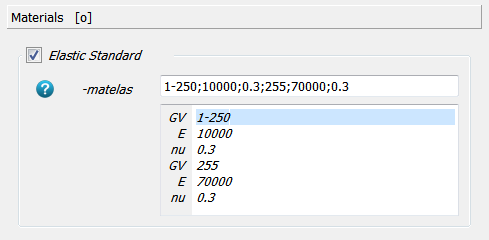
Next the material mapping is defined. The bone material is selected for gray values between 1-250 using
the -matelas option. Alternatively, a gray value dependent material could be defined using a
power law (-matpow option). The material is linear elastic and a Young’s modulus E and Poissons ratio
nu is provided.
A second material is added using the -matelas option to simulated a very rigid plate. Only
voxels with a gray value of 255 get this material behavior.
Note: The gray value of zero is reserved for “air” (no elements are created).
The automatic generation of node sets can be switched on in the Sets panel via the -nsetfa
option. In this way nodes from the bottom or top of the bounding box can be selected easily
via the names ALL_NODE_B and ALL_NODE_T.
Two boundary conditions are specified by using the -disp option. All DOFs (1-3) from the bottom nodes
(ALL_NODE_B) are fixed (0.0) and one DOF (3) from the top nodes (ALL_NODE_T) is moved
downwards by a given distance (-0.1).
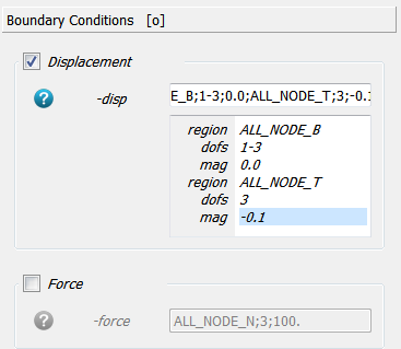
Note: This scripts creates a template file in the background denoted exa_temp.inp.
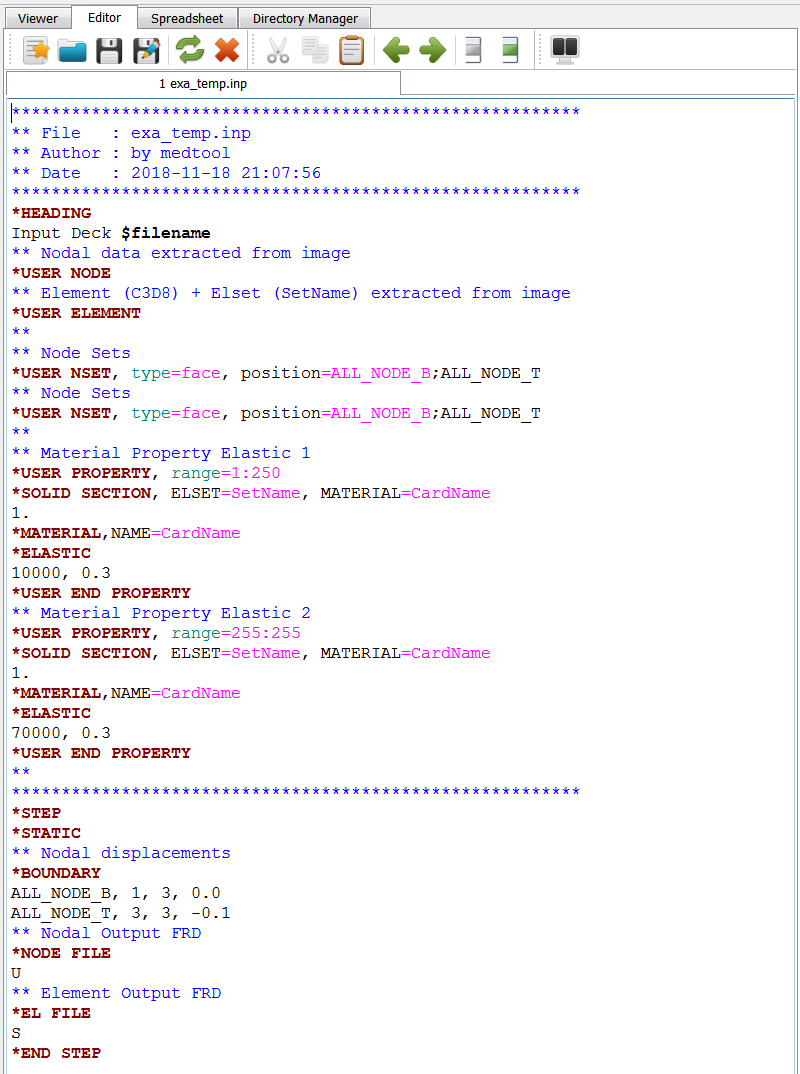
This file could be modified and used with Image - Processor -temp option to create an FEA input deck
with more flexibility.
Step 3
In this step of the medtool script, an Finite Element analysis is performed. This
example is tiny and should run on any PC quickly (less than 1min). The interface to Calculix (Solve - Calculix - ccx)
needs the previous generate input file (exa_main.inp).
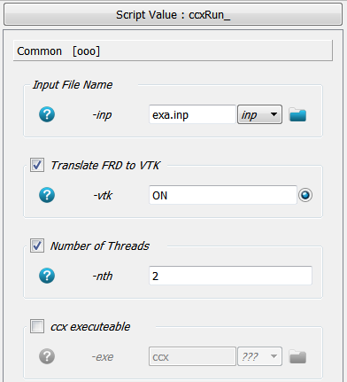
Furthermore, a VTK output is requested (-vtk) for Paraview and the solver should run on two threads (-nth).
Clicking the Run button sends a Calculix job to the system. Stopping the medtool scripts do not stop the Calculix run. This has to be done by hand using the Task Manageror a similar tool. After a successful run a file with the ending ‘.frd’ should be inside the working directory (takes around 30 secs in this example).
Notes: FEA is very CPU intensive and requires sufficient PC performance. If a ccx executable is given, check in advance if your Calculix versions is working correctly.
Step 4
The finite element results are check with Solve - Calculix - cgx (note the ‘g’ instead of an ‘c’). This allows to post-process the results. See the Calculix cgx help for more details.
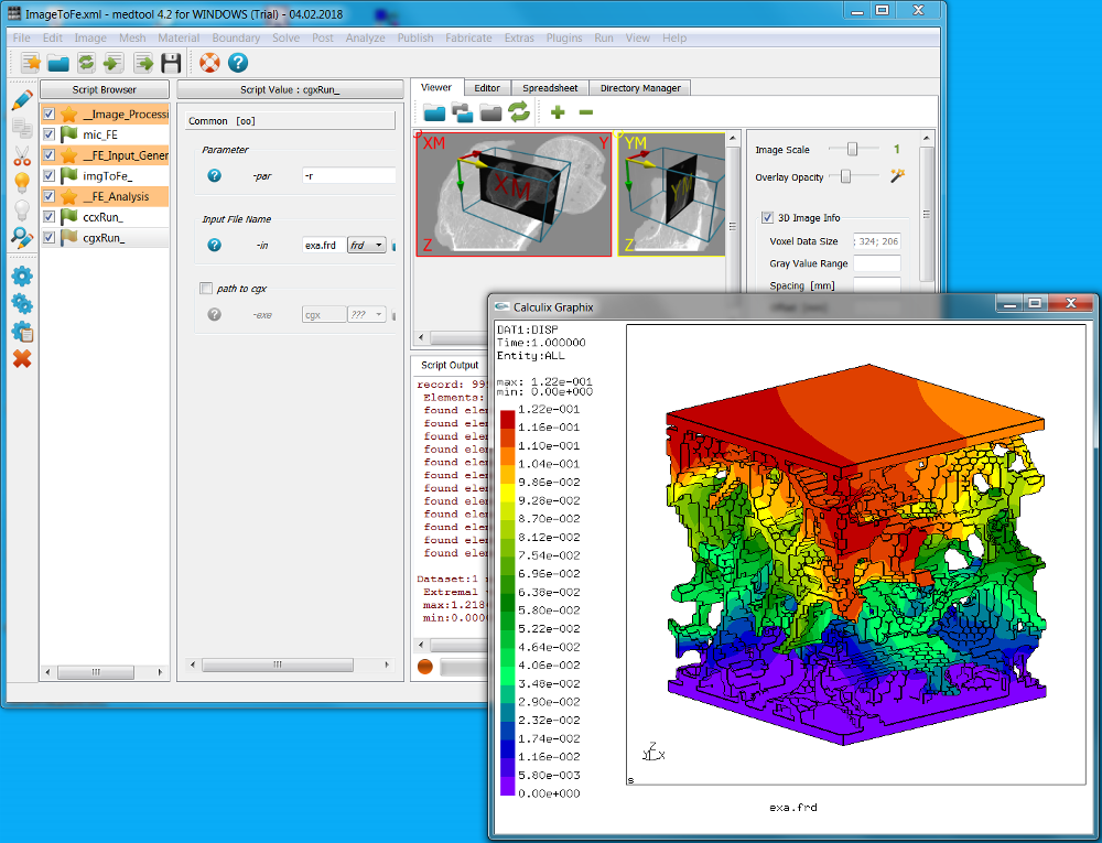
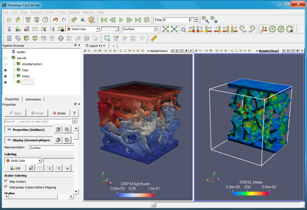
A second possibility to post-process the results is to use Paraview (not included in medtool but it is freely available from https://www.paraview.org/). The exported VTK file contains:
material IDs
scalar results (stresses)
vector results (displacements)
Step 2 and Step 3 could be also done with commercial FEA packages like Abaqus or the ‘.inp’ could be converted to any other FE format.
Image to Smooth Mesh (CGAL)
Note
User Level: Expert
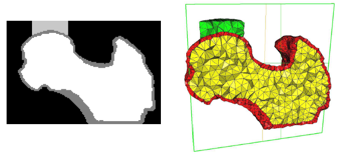
Simulation need grids (meshes) obtained from 3d image data. In this example the steps from a gray-level images to a 3d mesh are demonstrated. A direct gray-level domain mesher will be used to obtain the following results:
Two main steps are needed:
image processing (left picture) and
meshing (right picture).
The images processing consists of the following steps
cover the model by voxel layer
segment the full bone (outside)
segment the trabecular region (inside)
combine both and embed the model (labelled image for meshing)
mesh the model
convert the mesh to be able to view it with Paraview
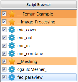
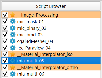
Finally the script browser will have the following look:
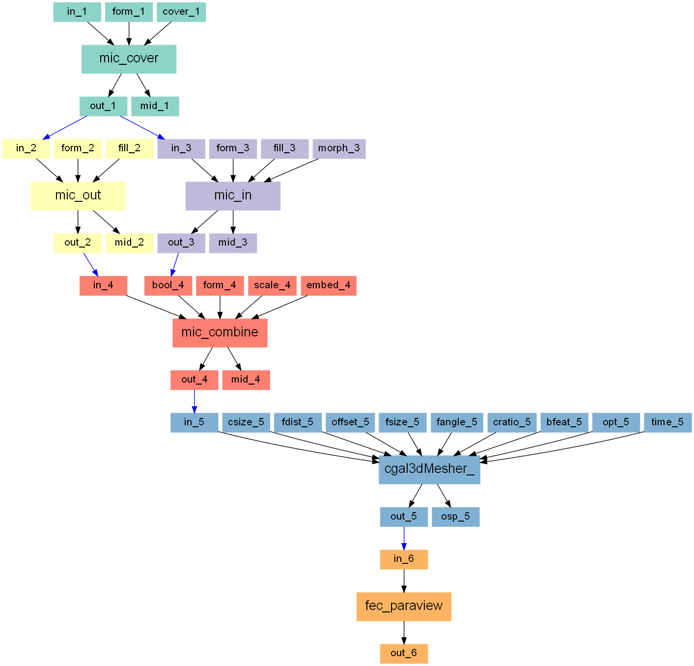
The entire workflow looks like this:
Please work through the example Image Processing before you start with this one.
Step 1
First, the original gray-level image is taken an a surrounded by a voxel
layer using Image - Processor and the option -cover by 5 voxels
witha gray-value of 0. In this way we
ensure that the bone is 100% inside because depending on the mesher voxels
at the boundary might be treated differently than inside voxels.
Step 2
The gray-level images is taken and the bone is segmented using from Image - Processor
the -fill option. This very powerful option extracts automatically the
outer (full bone), inner (trabecular) or thickness region based on a combination
of morphological and region growing steps. More details can be
found Pahr, D. H. & Zysset, P. K., CMBBE, 12, 2009. Play with the parameters
to see the effects.

Step 3
This step is the same as step 2 and used the -fill option but the inside
is extracted.

Step 4
In the last image processing step the inside and outside is combined using
the -bool option of Image - Processor. After scaling the images to
0..100 (-scale option) an embedding is added (-embed -option).
This image represents the labelled gray-value images for the mesher.

Step 5
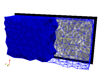
The image from step 4 is used in a mesher which is based on the CGAL library. Several parameters can be chosen to control the mesh. The cell size (overall element length) and the face distance (accuracy of surface representation) are the most important ones. Simply play with the others to fine tune the mesh.
Note: not properly set parameters may lead to holes in the cortex!
The output format is ABAQUS (‘.inp’). The 3D meshed as well as the 2D meshes (interfaces between the gray-levels) can be write out.
The content of the ‘.inp’ files shows this in more detail:
Step 6
For visualization reasons the files are converted to ‘.case’ using the Mesh - Converter. The resulting files can be view with Paraview. Alternatively, the ‘.inp’ file can be directly viewed with viewers like ABAQUS VIEWER, HyperMesh, etc.
The final results is shown in the following picture where part of the elements is masked to see also the inside.

FEA Material Mapping
Note
User Level: Standard
This example shows how to map bone elastic properties derived from CT images to a Finite Element mesh. An isotropic and orthotropic mapping example is shown. The input image is a high-resolution image to be able to get information about orthotropy. However, if only isotropic elastic properties are needed, also clinical or low-resolution images can be used. The results are viewed using Paraview.
The methodology demonstrated in here is described in more detail in:
Pahr & Zysset: Journal of Biomechanics, 2009, 42, 455-462 or
Gross, Kivell, Skinner, Nguyen, Pahr: Palaeontologia Electronica, 2014, 17.3
This demonstration is based on some basic knowledge on image processing (Image Processing ) and FE meshing (Image to Smooth Mesh (CGAL) ).
Before you continue reading, please open the medtool database (‘.xml* file) for this example. Change the working director to the unzipped directory by using Run Settings - Working directory. After this set up, no file paths need to be provided.
The following steps are demonstrated inside this example:
create an input trabecular CT image for orthotropic mapping
create an input trabecular CT image for isotropic mapping
mesh the region of interest
compute the isotropic and orthotropic material cards
visualize the results
The following scripts will be created:
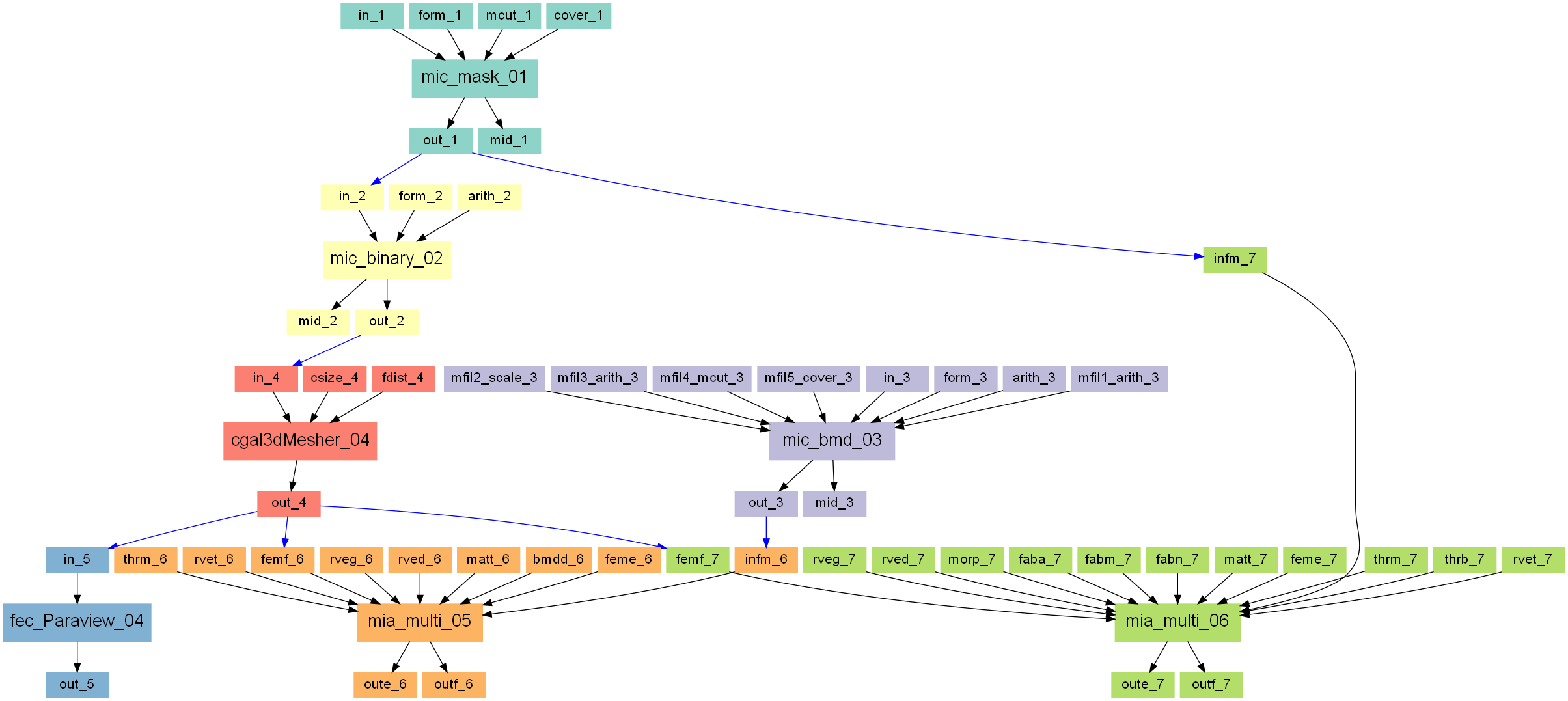
The entire workflow looks like this:
Step 1
Create an instance from Image - Processor by clicking on the menu entry.
The instance is called mic_mask_01. A 3D CT image of
trabecular bone is loaded, cropped (-mcut) and covered (-cover) by a
layer of seven voxel with a gray-value of 0. This step mimics a masked
image and would lead to more complex masks in reality. Note that the mask has
a value of 0 and all other gray-values are bigger than zero. This is important
in the following mapping step. The resulting images will be segmented and
is used for orthotropic material mapping. It looks like:
Step 2
In this step a binary images is created for the CGAL mesher. The -arith
option from Image - Processor is used to generate this image:
This image is used to mesh the ROI (white region).
Step 3
A slightly different image is needed for isotropic material mapping. In principle, the image from Step 1 could be used. However, it should be demonstrated later how a gray-level density image can be mapped without segmentation.
Background: A simple CT-value to bone mineral density (BMD) calibration is done.
Let’s assume bone mineral densities are ranging from 0-1060 mgHA/cc. Furthermore,
assume that a CT-value of 100-220 in the original CT image (matMapping.mhd)
corresponds to the bone densities of 0-1060 mgHA/cc.
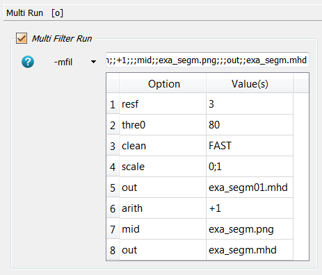
The -mfil option is used and looks like this:
The following multi run steps a done:
The CT-values are cut-off below 100 and above 220 using
-arithThe CT-values are scaled to 0-1060 to get the correct bone mineral densities
Bone densities of 0 are set to 1. This has nearly no influence on the mapping but otherwise, regions with 0 would not be considered in the mapping and treated as zero volume (ZV).
The image is cropped like in Step 1.
The image is covered with 0 like in Step 1. This is the ZV or “outside region. The mask has a gray-value of 0 and any value inside the ROI a value ranging from 1-1060 mgHA/cc.
Note
The calibration steps is much more complex and should be done via the Image - Calibrator script! It’s very important that no voxel inside the ROI has a gray-value of the mask (here 0).
The following image show the outcome of this step:
Step 4
CGAL is used to mesh the regions with gray-value 1. Standard parameters are used and the optimizer is switched on to avoid degenerated elements.
This mesh only covers roughly the ROI (trabecular bone).
Step 5
In order to view the previous the ‘.inp’ file from CGAL it is converted to ‘.case’ using Mesh - Converter. It could be directly viewed with an ABAQUS input deck viewer.
Step 6
Isotropic elastic material property mapping using the Material - CT Interpolator script:
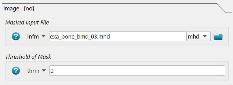
The -infm option points to the masked CT image file with the BMD values in it.
The mask is detected via -thrm option.
The size, shape, and distance of the background grid is given with the following options:
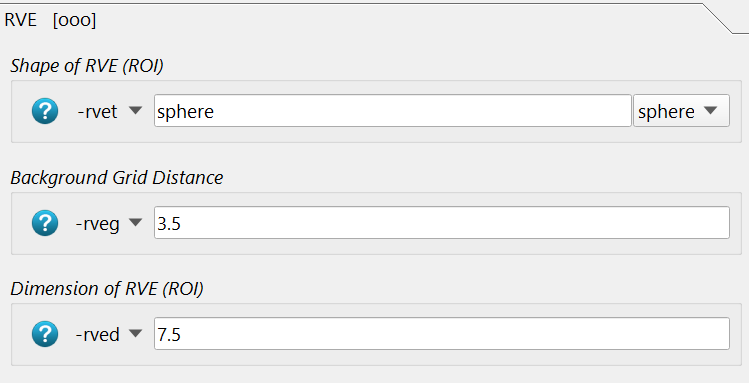
The background grid distance -rveg is 3.5mm and the sampling ROI size -rved is 7.5 mm.
Both are default parameters for human vertebra and femur. For smaller bones, smaller values
are needed (e.g. 2.5 and 5 mm).
Note
If you change these parameters, check the influence on the outcome!
Next we have to give all parameters for the isotropic mapping law:
These are:
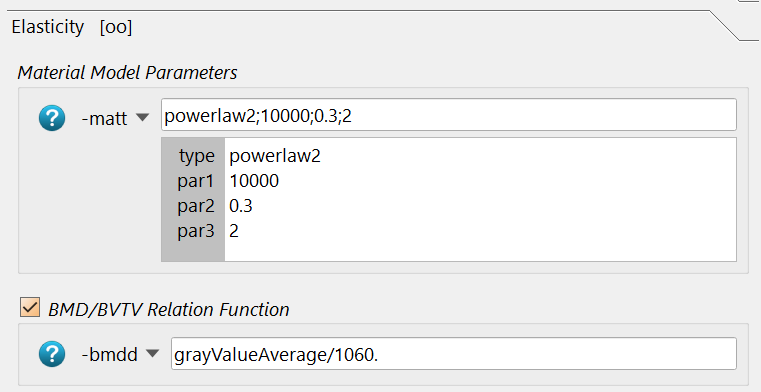
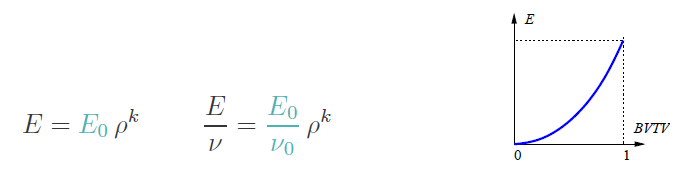
The type powerlaw2 (for powerlaw2 , the E module is 10000 MPa,
the Poisson ratio nu=0.3, and the power coefficient k=2.
Note
These parameters are assumptions and they may vary a lot for other studies!
A second entry in this panel is the -bmdd option. This is the formula
to compute the density \(\rho\) (ranging from 0…1) in the above
formula. The computed grayValueAverage inside the spherical 7.5mm
ROI is divided by 1060 mgHA/cc to obtain a density between 0 and 1. 0
means no bone, 0.5 means 50% bone, and 1. means 100% bone. Note that the
mask volume (or zero volume ZV), the total volume TV, and the bone volume BV
are connected to the density rho by:
rho = (BV)/(TV-ZV)
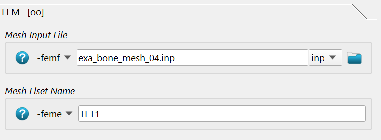
In the FEM section, the FE input deck -femf and the ELSET which should be
analyzed is given via -feme. The CGAL file is selected. Check the ELSET
in this file. This is the volume which gets the mapped values.
In this example the output is written to a AABAQUS/CALCULIX ‘.inp’ file
and to a ParaView/Ensight ‘.case’ file. Several other
output options would be possible for ABAQUS/CALCULIX using -outp,
-outf, -outs.
Many files are created which can be viewed with Paraview if the output format is ‘.case’.
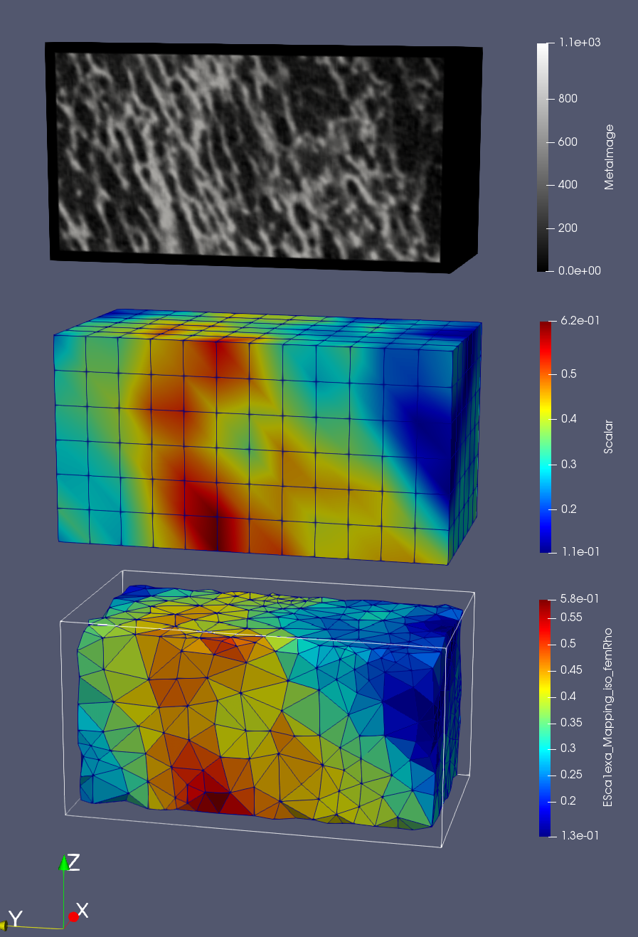
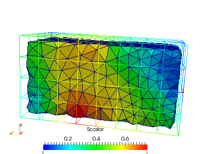
First the original density image is shown by loading the ‘exa_bone_bmd_03.mhd’ file into ParaView. Second, the files with the ending ‘_gridRho.case’ is shown which contains the values computed on the background grid (see papers for more info). The third images are the mapped and interpolated values on the given FE mesh (‘_femRho.case’ files). The colors represent the BV/TV. Good correlations between all images are visible.
Finally, we check the generated ABAQUS/CALCULIX ‘.inp’ file. This is important for FEA.
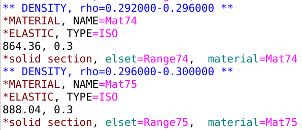
In case of a power law the number of written material cards can be controlled
via the -outn option. The default ist 250 material cards which is sufficient
for most cases and saves pre- and post processing time.
Note
The element type comes with the FE input deck. Change the element type aforehand (e.g. with Mesh - Converter) from linear to quadratic in case.
Step 7
Finally, the morphology is analyzed and mapped to orthotropic material cards by using Material - CT Interpolator. Most steps are like Step 6 and only differences are explained in detail.
First, the following parameters are given
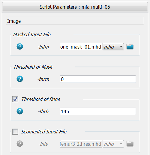
The -infm option points to the masked CT image file. The mask is detected
via -thrm. All voxels with this gray-values are treated as a mask. Therefore,
no voxel in the inside should have this value. Because a gray-level image is given, a
threshold -thrb is needed to segment the images e.g., to compute the fabric
i.e. orthotropy of the bone. A segmented image could be directly provided with -infs.
The RVE parameters -rveg and -rved are the same as in Step 6.
Additionally, some parameters could be switched on in the Fabric panel. These are default parameters and work most of the time. Please read the help for more details. If these parameters are not switched on, the same default parameters will be set.
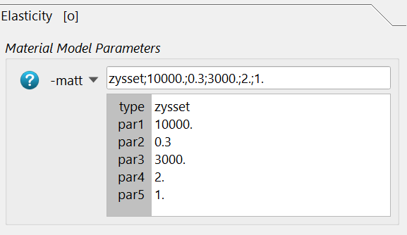
The Elasticity panel looks different from Step 6. In this step the orthotropic mapping law of Zysset 1995 is used:
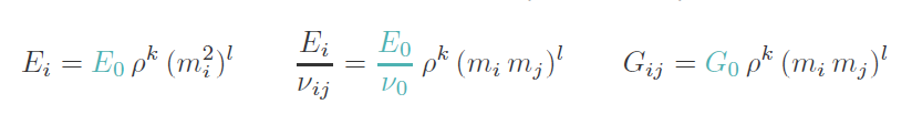
and the required parameters are inserted. Please read the help for more details.
The -bmdd option is not necessary because segmented images are used.
In the FEM and Output panels are the same as in Step 6. Only different file names are used.
During the run several warnings might appear like
** WARNING **: miaf77() Number of intersections = 0
which means the MIL algorithm does not find intersections. This usually happened if the analyzed volume is too small but is not a serious problem and can be changed by increasing the RVE size. Also, other warnings might pop up which should be checked carefully.
Many files are created which can be viewed with Paraview if the output format is ‘.case’. As described above, the files with the ending ‘_gridRho.case’ show the values computed on the background grid (see papers for more info).
The interpolation on the mesh can be seen by opening the ‘_femRho.case’ file. The colors represent the BV/TV.
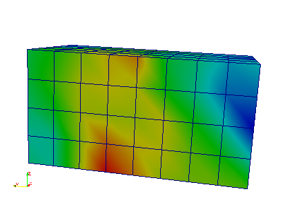
Additionally, the computed fabric orientations are in the files ‘_OrientMax.case’, ‘_OrientMid.case’, and ‘_OrientMin.case’. For example the maximum orientation for every FE element centroid are shown here:
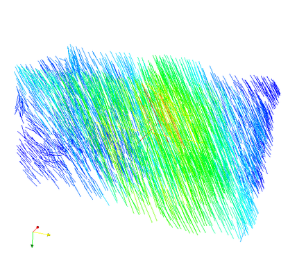
The value represents Young’s modulus in this direction. The agreement of both, the CT image and computed maximum orientation is show in the following:
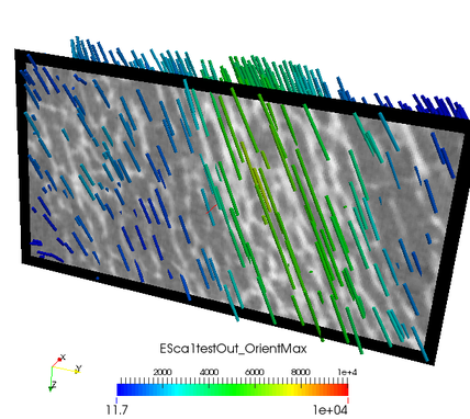
The values in these files correspond to Young’s modulus of the mapped material.
This information can be also written to ABAQUS (CALCULIX) input decks.
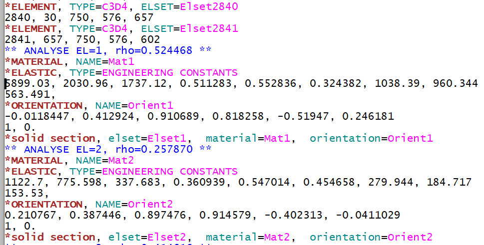
Compared to Step 6, ENGINEERING CONSTANTS plus an ORIENTATION is written for every element to represent orthotropic elastic material properties.
Note
During the mapping, for every element, a material card is written. Some pre- and post-processors have problems which such kinds of data because usually, only a few different material cards are inside a FE file. Therefore, keep your model small.
FEA Bone Homogenization
Note
User Level: Standard
One feature of medtool is the possibility to do computational homogenization. Shortly, it means that an in-homogeneous material (RVE) is meshed and analyzed in order to obtain the apparent stiffness tensor. More details can be found in:
Pahr & Zysset: Biomechanics and Modeling in Mechanobiology, 2008, 7, 463-476
This demonstration is based on basic knowledge of FE model generation with the Image - Processor (Image to FEA).
Before you continue reading, please open the medtool database (‘.xml* file) for this example. Change the working director to the unzip directory by using Run Settings - Working directory. After this set up, no file paths need to be provided. Please
This examples demonstrates how to:
generate the FE model
generate PMUBC and KUBC boundary conditions
run both models with CALCULIX
compute the homogenized stresses
compute the apparent stiffness tensors
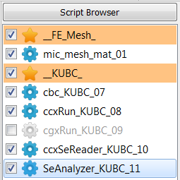
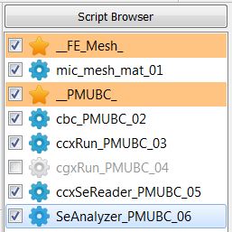
The following scripts will be created (two databases, one for KUBC and one for PMUBC):
The entire workflow looks like this:
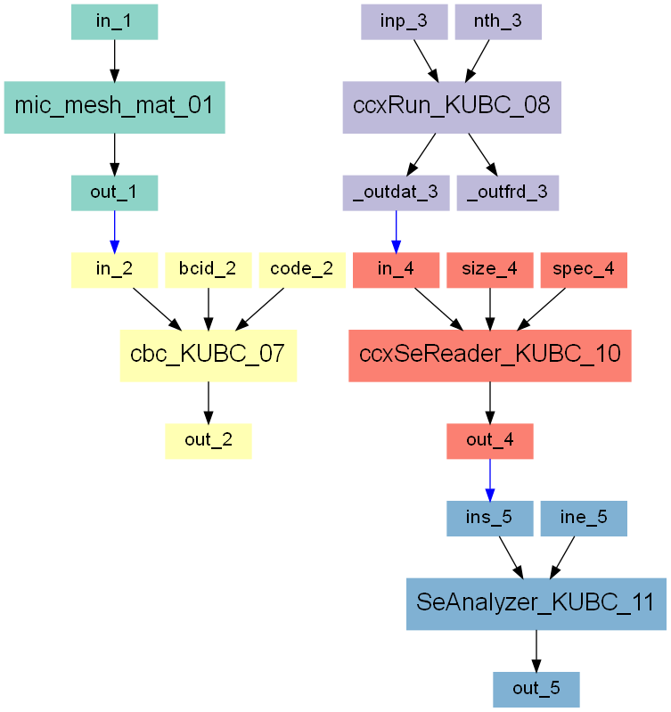
Step 1
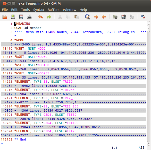
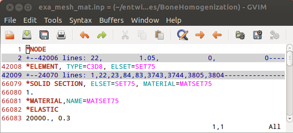
In the first step a segmented image of a 3x3x3mm bone cube is taken and meshed using Image - Processor. No template file is chosen and the automatically generated material parameters (E=20000 MPa, nu=0.3) are taken. For more flexibility with respect to this see Image to FEA . The obtained file contains the mesh (NODE, ELEMENT) and material definitions (MATERIAL, SOLID SECTION). An editor (e.g. gvim ) can be used to check the file content:
Step 2
The boundary conditions can be generated based on this mesh information. First periodic compatible mixed uniform boundary conditions (PMUBC) are generated using Boundary - BCs Generator script. The mesh is passed into the script and the output file is selected e.g. as ‘exa_bcs_PMUBC.inp’. The file is written in CALCULIX format and the SET option (NSET information at the boundary) is selected. Please check the file to see what is generated by the script.
Step 3
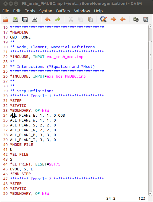
Before we can run CALCULIX a main input deck has to be written by hand or an example from Boundary - BCs Templates can be modified. The final file is provided as ‘FE_main_PMUBC.inp’. This file contains :
an INCLUDE statement for the mesh and material ‘.inp’ file
an INCLUDE statement for the boundary conditions ‘.inp’ file
six canonical loading steps which are uniaxial strain loading cases in this example
output statements to get element volumes and corresponding variables
It looks like this:
Step 4
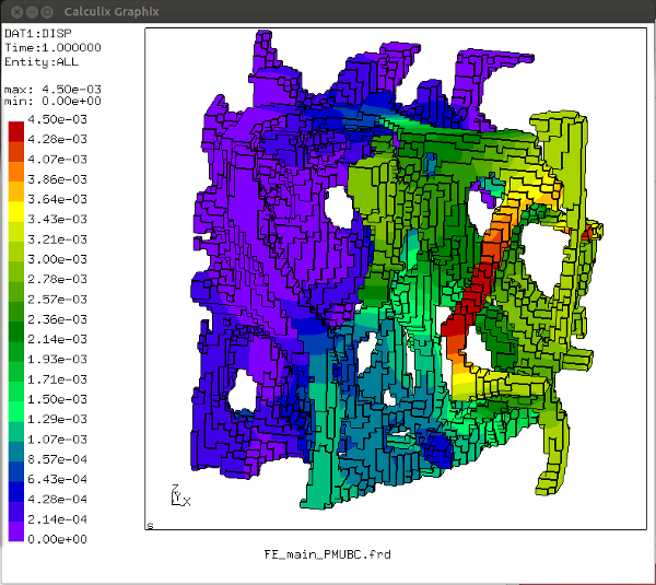
After the preparation of this file CALCULIX can be started with Solve - Calculix - ccx . A ‘.dat’ file including the element results and a ‘.frd’ for graphical post-processing is generated. Always look at the ‘.frd’ file first with Solve - Calculix - cgx or by directly calling cgx and check the deformations of the RVE for all six loading cases.
Step 5
First, the stresses has to be homogenized based on the FE results using Post - Calculix - SeReader2. This script reads the information from the CALCULIX ‘.dat’ file and writes the computed values to a text file (‘.out’). The output of this script reads as:
*STRESS
11 22 33 23 13 12  ** stress/strain component order
Step-1    +0.1577459    +0.0763435   +0.09858348  +0.002670643   -0.01343711   +0.01341488
Step-2    +0.0763435    +0.1778547    +0.1236368  -0.004793972   -0.01073155   +0.01960984
Step-3    +0.0985835    +0.1236368     +0.690022  -0.009596662   -0.03087805   +0.01803361
Step-4  +0.002628803  -0.001135259   +0.00253225  -0.005499516 -0.0008506188    +0.0280818
Step-5   -0.00313543 -0.0008168407   -0.01126357  +0.002518223   +0.04750546  +0.002529787
Step-6   +0.02354711   +0.00644126  +0.009929393   +0.09000341   +0.01002817  -0.002007178
These are volume averages of all stress components for each load case. Because we are using a porous media the same can not be done for the strains. An a-priori strain matrix has to be provides which looks like:
*STRAIN
11 22 33 23 13 12   ** stress/strain component order
tens1    0.001  0.000  0.000  0.000  0.000  0.000
tens2    0.000  0.001  0.000  0.000  0.000  0.000
tens3    0.000  0.000  0.001  0.000  0.000  0.000
shear12  0.000  0.000  0.000  0.000  0.000  0.001
shear13  0.000  0.000  0.000  0.000  0.001  0.000
shear23  0.000  0.000  0.000  0.001  0.000  0.000
and is located in the ‘apriori-STRAIN.txt’ file inside the example folder. The reason is because the volume averaging would not yield the correct results. See the above paper for more details.
Step 6
These two files (STRESS and STRAIN averages of six load cases) can be used to compute the homogenized material behavior using Post - SeAnalyzer. This script gives the following output:
===============================================================================
    H O M O G E N I Z E D  Elastic Properties from FEM models
===============================================================================
STRESS Input = exa_PMUBC_STRESS.out
STRAIN Input = apriori-STRAIN.txt
Output File  = exa_PMUBC_HOMOG.out
Method       = Stress/Strain Volume Averaging
Date - Time = 2014/11/2 - 10:9

Averaged Strains
===============================================================================
Step      E11          E22          E33          E12          E13          E23
-------------------------------------------------------------------------------
1 +1.0000e-03  +0.0000e+00  +0.0000e+00  +0.0000e+00  +0.0000e+00  +0.0000e+00
2 +0.0000e+00  +1.0000e-03  +0.0000e+00  +0.0000e+00  +0.0000e+00  +0.0000e+00
3 +0.0000e+00  +0.0000e+00  +1.0000e-03  +0.0000e+00  +0.0000e+00  +0.0000e+00
4 +0.0000e+00  +0.0000e+00  +0.0000e+00  +1.0000e-03  +0.0000e+00  +0.0000e+00
5 +0.0000e+00  +0.0000e+00  +0.0000e+00  +0.0000e+00  +1.0000e-03  +0.0000e+00
6 +0.0000e+00  +0.0000e+00  +0.0000e+00  +0.0000e+00  +0.0000e+00  +1.0000e-03


Averaged Stresses
===============================================================================
Step      S11          S22          S33          S12          S13          S23
-------------------------------------------------------------------------------
1 +1.5775e-01  +7.6343e-02  +9.8583e-02  +1.3415e-02  -1.3437e-02  +2.6706e-03
2 +7.6343e-02  +1.7785e-01  +1.2364e-01  +1.9610e-02  -1.0732e-02  -4.7940e-03
3 +9.8584e-02  +1.2364e-01  +6.9002e-01  +1.8034e-02  -3.0878e-02  -9.5967e-03
4 +2.6288e-03  -1.1353e-03  +2.5323e-03  +2.8082e-02  -8.5062e-04  -5.4995e-03
5 -3.1354e-03  -8.1684e-04  -1.1264e-02  +2.5298e-03  +4.7505e-02  +2.5182e-03
6 +2.3547e-02  +6.4413e-03  +9.9294e-03  -2.0072e-03  +1.0028e-02  +9.0003e-02


*******************************************************************************
*STIFFNESS Matrix
11 22 33 23 13 12      ** stress/strain component order
2                      ** symmetrization factor (2..engineering)
*******************************************************************************
      +157.7       +76.34       +98.58       +23.55       -3.135       +2.629
      +76.34       +177.9       +123.6       +6.441      -0.8168       -1.135
      +98.58       +123.6         +690       +9.929       -11.26       +2.532
      +2.671       -4.794       -9.597          +90       +2.518         -5.5
      -13.44       -10.73       -30.88       +10.03       +47.51      -0.8506
      +13.41       +19.61       +18.03       -2.007        +2.53       +28.08


*******************************************************************************
*COMPLIANCE Matrix
11 22 33 23 13 12      ** stress/strain component order
2                      ** symmetrization factor (2..engineering)
*******************************************************************************
    +0.00839    -0.003055   -0.0006235    -0.001993   +0.0005244    -0.001227
    -0.00317    +0.007534   -0.0009269   +0.0004501   -0.0003639    +0.000762
  -0.0005936    -0.000902    +0.001715   -1.221e-05   +0.0003593    -0.000127
  -0.0006161   +0.0001946   +0.0001195     +0.01138   -0.0007324    +0.002261
  +0.001373   +0.0001528   +0.0006999    -0.002841     +0.02146   -9.165e-05
  -0.001581    -0.003222   -0.0002106    +0.001715    -0.002213     +0.03592


ENGINEERING Constants
===============================================================================
  E_1 =       119.19     |  G_23 =       87.898      | nu_23 =      0.11972
  E_2 =       132.73     |  G_13 =       46.588      | nu_13 =     0.070747
  E_3 =       583.13     |  G_12 =       27.843      | nu_12 =      0.37786
Note that the script Analyzer - Stiffness - Concatenator can be used to write this information in a comma separated file (CSV) for the use with a spreadsheet software. This script allows also an append mode such that many homogenization results can be written in one CSV file.
Step 7-11
These steps are similar to step 2-5. The difference is that kinematic uniform boundary conditions (KUBCs) are used. This gives an other set of apparent stiffness quantities as summarized in the following:
===============================================================================
    H O M O G E N I Z E D  Elastic Properties from FEM models
===============================================================================
STRESS Input = exa_KUBC_STRESS.out
STRAIN Input = apriori-STRAIN.txt
Output File  = exa_KUBC_HOMOG.out
Method       = Stress/Strain Volume Averaging
Date - Time = 2014/11/2 - 10:10

Averaged Strains
===============================================================================
Step      E11          E22          E33          E12          E13          E23
-------------------------------------------------------------------------------
1 +1.0000e-03  +0.0000e+00  +0.0000e+00  +0.0000e+00  +0.0000e+00  +0.0000e+00
2 +0.0000e+00  +1.0000e-03  +0.0000e+00  +0.0000e+00  +0.0000e+00  +0.0000e+00
3 +0.0000e+00  +0.0000e+00  +1.0000e-03  +0.0000e+00  +0.0000e+00  +0.0000e+00
4 +0.0000e+00  +0.0000e+00  +0.0000e+00  +1.0000e-03  +0.0000e+00  +0.0000e+00
5 +0.0000e+00  +0.0000e+00  +0.0000e+00  +0.0000e+00  +1.0000e-03  +0.0000e+00
6 +0.0000e+00  +0.0000e+00  +0.0000e+00  +0.0000e+00  +0.0000e+00  +1.0000e-03


Averaged Stresses
===============================================================================
Step      S11          S22          S33          S12          S13          S23
-------------------------------------------------------------------------------
1 +4.7062e-01  +1.7657e-01  +1.8524e-01  +7.2569e-02  -3.4966e-02  -7.4421e-03
2 +1.7657e-01  +5.3374e-01  +2.2830e-01  +5.4050e-02  -2.0209e-02  -1.9869e-02
3 +1.8524e-01  +2.2830e-01  +1.0128e+00  +3.1827e-02  -5.4834e-02  -1.0639e-02
4 +7.2569e-02  +5.4050e-02  +3.1827e-02  +1.7207e-01  -5.9078e-03  -1.5791e-02
5 -3.4966e-02  -2.0209e-02  -5.4834e-02  -5.9078e-03  +1.8768e-01  +3.4144e-02
6 -7.4421e-03  -1.9869e-02  -1.0639e-02  -1.5791e-02  +3.4144e-02  +2.4574e-01


*******************************************************************************
*STIFFNESS Matrix
11 22 33 23 13 12      ** stress/strain component order
2                      ** symmetrization factor (2..engineering)
*******************************************************************************
      +470.6       +176.6       +185.2       -7.442       -34.97       +72.57
      +176.6       +533.7       +228.3       -19.87       -20.21       +54.05
      +185.2       +228.3        +1013       -10.64       -54.83       +31.83
      -7.442       -19.87       -10.64       +245.7       +34.14       -15.79
      -34.97       -20.21       -54.83       +34.14       +187.7       -5.908
      +72.57       +54.05       +31.83       -15.79       -5.908       +172.1


*******************************************************************************
*COMPLIANCE Matrix
11 22 33 23 13 12      ** stress/strain component order
2                      ** symmetrization factor (2..engineering)
*******************************************************************************
  +0.002639   -0.0006527   -0.0002921   -8.528e-05   +0.0003247   -0.0008505
  -0.0006527    +0.002296   -0.0003865   +0.0001288   -2.223e-05   -0.0003632
  -0.0002921   -0.0003865     +0.00114   -2.183e-05   +0.0002421   +4.012e-05
  -8.528e-05   +0.0001288   -2.183e-05    +0.004205   -0.0007621   +0.0003593
  +0.0003247   -2.223e-05   +0.0002421   -0.0007621    +0.005594   -5.263e-05
  -0.0008505   -0.0003632   +4.012e-05   +0.0003593   -5.263e-05    +0.006308


ENGINEERING Constants
===============================================================================
  E_1 =       378.98     |  G_23 =        237.8      | nu_23 =      0.16838
  E_2 =       435.62     |  G_13 =       178.76      | nu_13 =      0.11069
  E_3 =       877.55     |  G_12 =       158.52      | nu_12 =      0.24737
XY-Plotting
Note
User Level: Standard
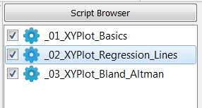
This example demonstrates the capabilities of the XY-Plotter script.
Following working steps are done inside this example:
check an xy data file
make an xy scatter plot of two datasets
plot the regression line including regression results
create Bland-Altman plots from these data sets.
The final medool database looks like:
Start first with a blank XY Plotter script, try to do each step by your own and check out the full example script afterwards.
Step 1
A CSV data file is needed by the scripts. There is one file in the example
folder named data.csv. Alternatively, such a data file could be generated
with a spreadsheet software. The content of the file can be viewed with the
Editor in medool:
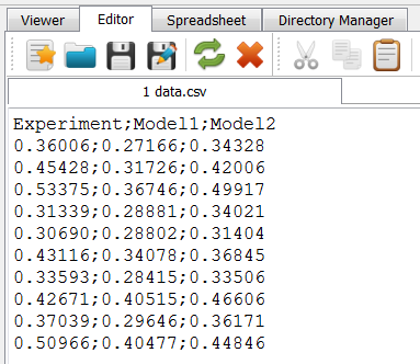
The file contains one header line and three data columns showing 10 data lines.
Step 2
An xy plot script is created by clicking on Publish - XY Plotter. After creation following options are edited inside the Common panel:
First go to
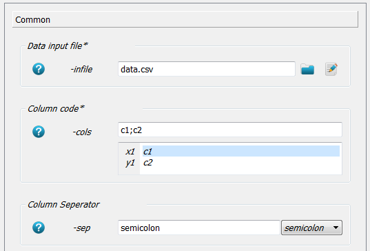
-infileand select thedata.csvfile. No path is given because the working directory was set accordingly as in the above examples.Next column 1 should act as x and column 2 as y axis. Therefore,
c1;c2;is written in the-colsoption.The column separator is chosen with
-sepoption assemicolon(i.e. a;in the data file).
Step 3
Next the script is executed by clicking the Run Active … button. Following warning messages pop up:
**WARNING** -line and/or -marker type not chosen. Data are not plotted!

**WARNING** -pyplgui and/or -plotfile not chosen. No GUI window or plot file generated!

**WARNING** Unable to read line: Experiment;Model1;Model2
They have following meaning:
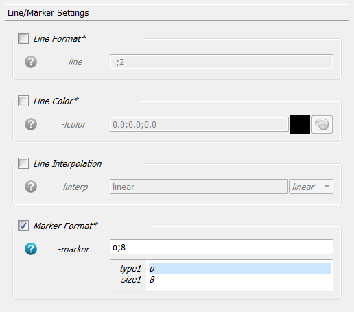
under Line/Marker Settings panel the option
-lineor-markerneeds to be selected otherwise nothing is plotted. We select-markeraso;8. This means circles (oletter) are drawn with a size of 8. For more details check out http://matplotlib.org/ .
-pyplguiand/or-plotfileneeds to be given to produce output. We select-pyplguitoONto get an interactive window. Using-plotfilewould print the output on a file without the need to open the plot window. This is very helpful for parameter runs.The first line in our dataset is a heading line which can not be interpreted. Switch
-nheader(number of header lines) on and give as value1to over read the first line. The Common and Line/Marker Settings panel looks like: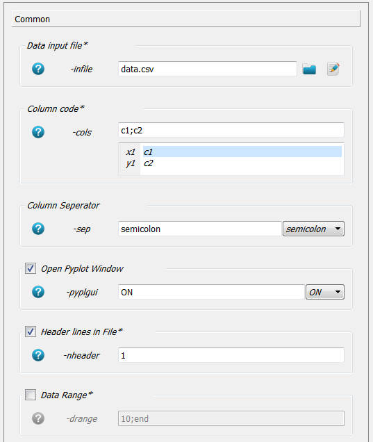
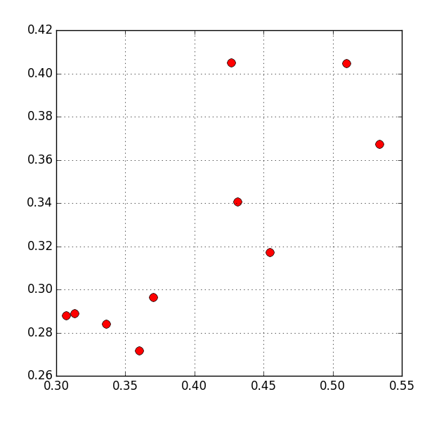
Re-running the script shows a simple xy-plot:
Step 4
A second data set is added in this step. More option values need to be added in
fields which are indicated by * at the end of the option description like
Data input file* in case of the -infile option.
This means:
Go to
-infileand select two datafilesdata.csv;data.csv. Here we have twice the same file name but the second plot could also be generated from an other data file.Go to
-colsand type inc1;c2;c1;c3to plot column 2 and column 3 over column 1.Go to
-nheaderand type in1;1to over read twice the headers.Go to
-markerand choose0;8;v;8to select circles (o) and triangles (v) with a size of 8.
The script throws an error if not all options with a * are edited accordingly.
Re-running the script shows an xy-plot with two data sets in it:
Step 5
There are many possibilities to change the style of a plot. In this example following improvements are done:
An annotation is given by activating the
-atableoption inside the Annotation panel.The Figure and Axes Settings are changed i.e. the x and y limits (
-xlim,-ylim), axes labels are given (-axlabel), a legend text (-legend) is actived, and a title for the plot (-title) is added.The Fontsize panel is used to change the font size e.g.
-fntsztlfor the title.
Further options like colouring, plot style, etc are possible. The final output of the first XY Plotter script looks like:
Step 6
In this step regression lines are added to the previous plot which gives the following plot:
For this task the previous XY Plotter script is copied and modified. Following steps are needed to create such a picture:
Go to the Regression Line panel and edit
-reglineto give the thickness of the regression line.1;1means a thickness of 1 for both data sets. This option activates the plotting and the computation of the regression data.Check the
-reglegendoption and give the legend text. This text is plotted only if the-legendoption is active. Following entries are given as legend text:EQN, R2, SEE;EQN, R2, SEE
where
EQNis replaced by the regression equation,R2is replaced by the squared Pearson correlation coefficient, andSEEis replaced by the standard error of the estimated. Also additional text can be given (here only blanks and commas). In this way the legend can be fully customized by the user.In Figure and Axes Settings the axis limits, grid appearance (
-grid), and labels are changed as visible in the above plot.
Step 7
In this step a Bland-Altman plot as show in the figure below is created.
For this task the first XY Plotter script is copied and modified. Following steps need to be done to create such a picture:
The
-colsoption is modified such that(c1+c2)/2;(c1-c2);(c1+c3)/2;(c1-c3)
in order to compute the mean and difference of the two measures as defined by Bland-Altman.
In the Bland-Alman Lines panel
-balineis activated to plot the lines for the mean and 1.96 SD (standard deviation) lines. the two numbers1;1give the line thickness of these lines for the first and second dataset.The
-balegendis activated and the text for the legend is giving including replacement symbols. EspeciallyLB,AVG, andUBare replace by computed values for the lower bound (mean - 1.96 SD), the mean, and the upper bound (mean + 1.96 SD) of the data difference of 2 measures.
Report Making
Note
User Level: Standard
This example demonstrated how to make an automated report with medtool. As example the influence of a segmentation with different thresholds (70/80/90) is investigated and summarized in a report.
Following working steps are done inside this example:
generate segmented data for a report
make a 3D rendering of the sample for a report
merge two parameter files
make a PDF report with the above data
The final medtool database needs to be run in 3 steps:
Select all scripts under
__Data_Param_Run_1_, deselect all scripts and Run Parameter Study ….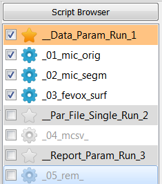
Select the script under
__Par_File_Single_Run_2_, deselect all scripts under and Run Active ….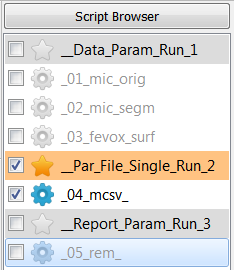
Select the script under
__Data_Param_Run_3_, deselect all others and Run Parameter Study ….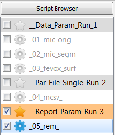
These three steps are necessary because the first run generates data for the parameter file, the second runs appends the data to a parameter file, and the third creates the report.
Step 1
The image file and processing steps are the same as used in the Image Processing example. Please look up details there. In this example we explore the underlying image data file by
creating a script named
_01_mic_origwith Image - Processorselecting the data file name (
-in) from the example calledspongyBone5.mhdactivating the mid-plane option
-midand giving a filename e.g.exa_orig.pngrunning this script in Run Active … mode.
These steps read the image and write midplanes (exa_orig-XM.png, …) which can be viewed with
the Viewer and will be used later.
Step 2
Next, the data file is segmented with varying threshold values. Therefore, a parameter
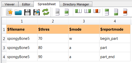
file is needed. It comes with this example and shows the following content:
(spongy.csv):
Following steps are done to segment the image:
Create an Image - Processor script called
_02_mic_segm.Change
-intospongyBone5.mhd,-outtoexa_segm_$thres.mhd, and-midtoexa_segm_$thres.png. Note that the parameter$thresis used inside the filename. In this way new files are generated during each parameter run.Go to the Segmentation Filter panel and give the parameter
$thresfor the-thre0option.Activate
-cleanin the Modify Filter panel to avoid unconnected regions.Select in the Image Info panel the option
-ifotoexa_info.csv;$mode. This writes a CSV file using the parameter$modeas output mode. In this way the first run writes the header and first data line withwand in all other runs append data lines (lettera).Check in Run Settings that
spongy.csvis selected as parameter file.Run the
_02_mic_segmscript with the Run Parameter Study … option.
Although the first script contains no parameters it is re-run for convenience. Beside the segmented mid-plane files (see figure)
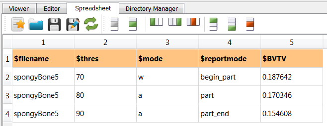
also a file which can be used as parameter file (exa_info.csv) with following content is generated:
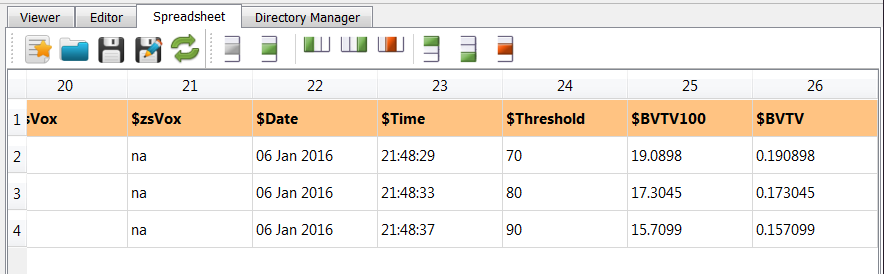
For example, at the very end of the file we see $BVTV - the bone density - as useful output.
This output will be used later on for the report.
Step 3
In this step a 3D rendering of the bone is created which will be also used in the report. The Fabricate - 3D Print allows to create renderings of iso-surfaces.
- Following steps are done to render the image. First go to the Common panel to
Select the segmented image file via
-finand select the fileexa_segm_$thres.mhd.The interactive view window (
-showoption) should be switchONfor checking but is usually switchedOFFduring a parameter run.Got to the Output panel and select
-scrxyzoption to create three orthogonal screenshots.
Running the script shows the following interactive window:
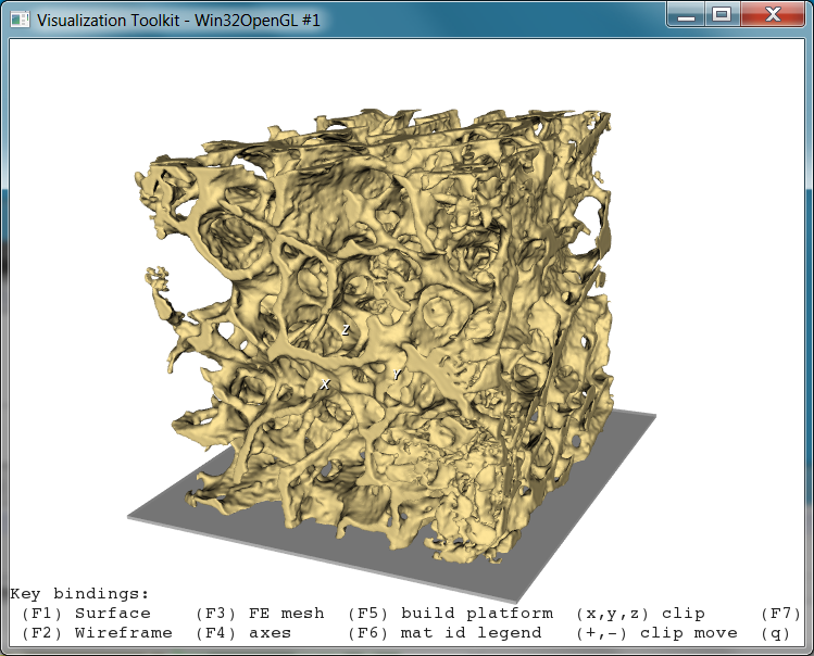
This 3D rendering could be improved by -smooth, reduced by -decim, and also stored e.g. in STL format
for 3D printing.
Finally, run this or all scripts under the __Data_Param_Run_1 as parameter study.
Step 4
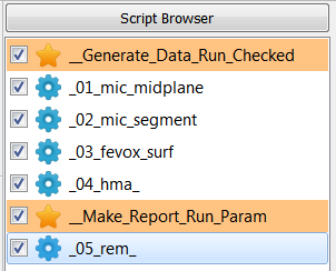
Deactivate the __Data_Param_Run_1 scripts and activate the __Par_File_Single_Run_2
script. The following is visible in the Script Browser:
Before the generation of a report the parameter file (spongy.csv) is extended by the BVTV parameter
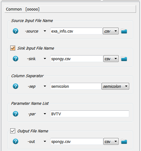
from Step 2. The Extras - File - CSV Merger script is able to do this automatically. After script creation the Common panel
of the _04_mcsv_ script is modified accordingly:
Modifications notes:
A source file
-sourceis given from where data columns are read. This file was generated in Step 2.A sink file
-sinkis provided where the data columns are replaced or appended.A separator needs to be given which is usually
;(a semicolon) in medtool.A parameter name (column name in
exa_info.csv) is given which should be read. Here the parameter$BVTVis read from this file. Note that the$sign must not be given!At the end the modified
-sinkfile is overwritten but also a new file could be created.
After running this script with Run Active … the following spongy.csv file is obtained:
It is visible that a column was append and the rest was kept unchanged. This script could be deactivated now.
However, it should be noted that in this case the file is not updated if more parameters are added or the threshold
$thres are changed.
Step 5
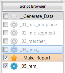
Deactivate the __Par_File_Single_Run_2 and activate the __Report_Param_Run_3 scripts.
The following is visible in the Script Browser:
In the last step a PDF report is created using the script Publish - Report Maker.
The basic idea is to give the data e.g. a Title,
Text, Equation, Figure, and Table column of the script in separate entries and to define
a layout in a packing table (-pack). In this example the packing looks like:
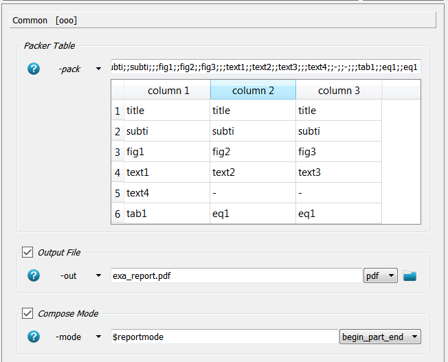
A 6x3 table is defined. The first row is covered by the title which is given in the -title option.
The same holds for the second row - the subtitle.
In the third row three figures are distributed equally where the file names are given in the
-fig1, -fig2, and -fig3 option of this script. The same holds for the text and table entries.
The output file is given in the -out option which is a PDF file. It should be noted that the script
creates a latex file in the background and compiles this file with pdflatex. Under Window this requires
a MikTeX installation. (https://de.wikipedia.org/wiki/LaTeX, for a 30 min tutorial see
http://lotfi.net/latex/learn_latex.pdf). If the portable editon is installed (see
http://miktex.org/portable ) the path to the pdflatex file can be given in the -pdflatex option. In this
way Latex styles (e.g. \bf{..} as bold font etc) can be used in text, equation, and table entries.
One more important thing is the -mode option. Because multiple pages are generated after every run only a piece of
the latex file is generated and the PDF is generated after the final run. Therefore, the parameter $reportmode is
need which is given in the parameter file (see above).
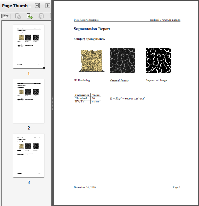
In the Settings panel a few more options like a header title and figure size is defined. Now the script is ready for a Run Parameter Study …. A PDF file is created which contains 3 pages:
CT Bone Morphometry
Note
User Level: Standard
This example shows how CT-derived bone morphometry can be performed with medtool. The input to the analyser is a 3D CT image. Morphometric measurements are performed in order to give estimates for variables like trabecular thickness (Tb.Th), spacing (Tb.Sp), density (BV/TV), volumes (BV), surfaces (BS), orientations of the bone (DA), etc. These measurements can be summarized in an automatically generated PDF report.
Following working steps are done inside this example:
generate segmented data for a report
make a 3D rendering of the sample for a report
do a CT-derived bone morphometric analysis and export the data
make a PDF report with the computed data
The final medool database looks like this:
It is recommended to do the example Report Making before doing this one.
Step 1
This step is very similar to the one in example Report Making and should be look up there. A mid-plane image is generated by this scripts using Image - Processor.
Step 2
The _02_mic_segm_ script creates an image which is needed by the Analyze -
CT Morphometry script. It must have 3 gray-values:
2 for the bone
1 for the marrow
0 for everything else which is outside the volume of interest (VOI). In this example the full cube is the VOI. Thus, there is no 0 value.
Please read the documentation of the Analyze - CT Morphometry script for more details.
For convenience the generation of such an image is done via the
multi run option (-mfil in Image - Processor). The corresponding panel looks like:
Shortly the image is resized by a factor of 3 (resf) in order to speed up
the analysis in this example but this should not be done in real analysis. In
the next step the image is thresholded (-thres) and cleaned (-clean) to
remove unconnected regions. Then it is scaled (-scale) to 0-1. This image
is stored (-out) and used in the script _03_fevox_surf_. Afterwards,
a value of 1 is added to the image (-arith) to get an image with 1 for
marrow and 2 for the bone region. Finally, everything is written into
files namely -out for the script _04_hma_ and -mid for the script _05_rem_.
Step 3
This step is again very similar to the one in example Report Making. A 3D rendering is generated by this scripts using Fabricate - 3D Print to extract the iso-surface. Shortly
set
-fintoexa_segm01.mhd(image with two gray-values used to extract the iso-surface)set
-ciftospongy.cam(a file which contains a camera positions for an isometric view)set
-screentoexa_3D.png(iso-surface rendering for the report)
Step 4
This is the main step for doing the morphometric analysis. A script is
loaded via the Analyze - CT Morphometry menu and renamed as __04_hma_.
Following sub-steps are done inside this script:
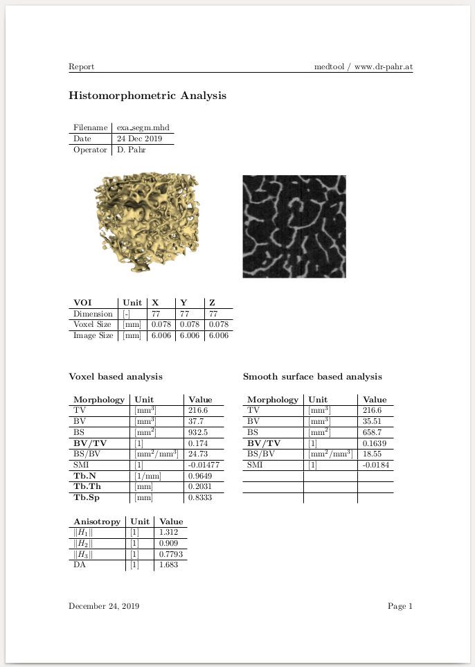
An input file name (
-in=exa_segm.mhd) is given to select the 0/1/2 gray-level image.The requested output data are activated. In this example only quantities from the Trabecular panel are used. Check out guidelines for CT-derived morphology here: https://www.ncbi.nlm.nih.gov/pubmed/20533309
The
-outoption is selected in the Output Option panel and a CSV file calledexa_hma.csvwill be written. The content of this file is a standard medtool parameter file: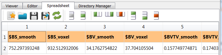
Step 1-4 should executed in the Run checked … mode because it is a single analysis.
Step 5
After running the previous steps all data are ready to generate a report. The procedure is similar as the one presented in the Report Making example. Following steps are done:
Open the
exa_hma.csvfile from Step 4 and check out the available parameters. This file contains all parameter which are used in this report.Create a Report Maker script called
05_rem_.Setup this script as explained in the Report Making example.
Select
exa_hma.csvas parameter file in the Run Settings area.Select only this script i.e.
Run the Report Maker script called
05_rem_in Run Parameter Study … mode to generate the PDF file. This is required to replace the parameters by the real values.
Finally the following output PDF file is produced:
This procedure can be simply extended to run a parameter study as shown in the Report Making example.
CT Bone Morphometry Mapping
Note
User Level: Standard
The example CT Bone Morphometry investigates a single (small) volume of interest. Since medtool version 4.4, the Analyze - CT Morphometry script allows multiple morphological analyses based on automatically created ROIs.
This functionality and the used data of this example is similar to the one explained
in the example FEA Material Mapping. Compared to the script Material - CT Interpolator,
this script is not limited to BVTV and DA and has following additional
features:
all availabe morphometry parameters can analyzed
simplifed usage
multiprocessing is possible
This examples demonstrates how to:
check the segmented input image
create a mesh that covers the analysis region
perform a bone morphometry mapping
The following scripts will be created:
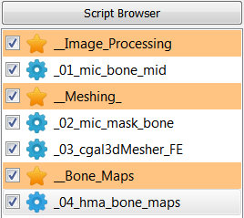
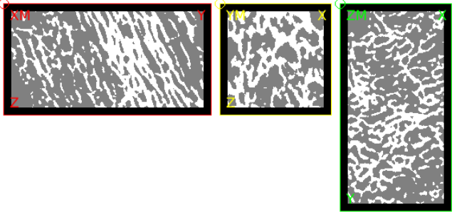
Step 1
In the first step, the input image is checked by an Image - Processor script. An approximately 20x20x40mm large embedded bone piece serves as input. Note that the bone has the gray value 2, marrow the gray value 1, and regions that are not to be analyzed have a gray value of 0.
Step 2
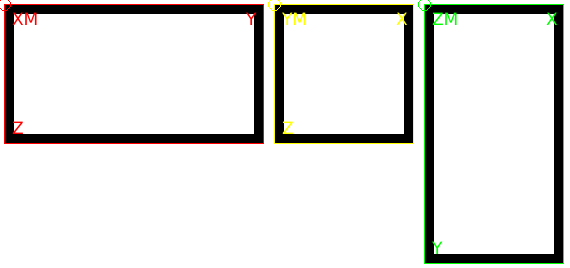
In the second and third step, we create a mesh that encompasses the analysis area (i.e., forms the interface to the gray value 0). However, the mesh does not have to be generated for bone map analysis. More details will be explained later.
An Image - Processor script (_02_mic_mask_bone) is used to create a 0/1 mask
of the analysis area with the -arith option.
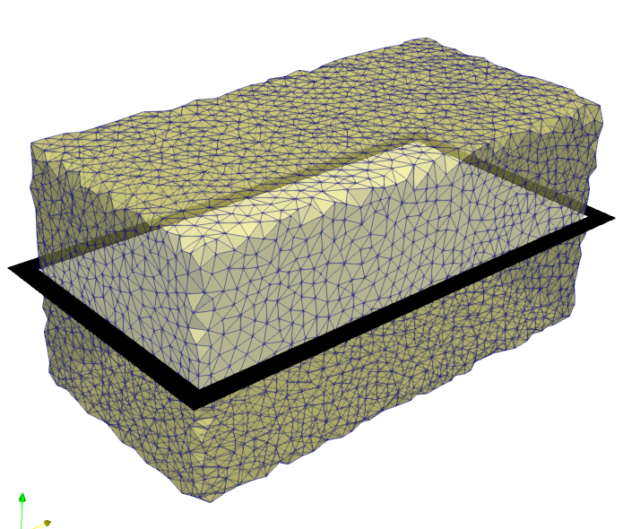
Step 3
Subsequently, a volume mesh is generated with this mask using Mesh - 3D - CGAL Mesher
(_03_cgal3dMesher_FE). The obtained mesh is usuallyused in finite element (FE)
analyzes. Here it serves only to visualize the results.
In this example, an image is used which has an offset other than 0/0/0.
For this reason, the option -offset is activated in the mesher. By default,
CGAL ignores offsets in image files.
A visual check of the offset can be done with Paraview by loading the mesh and the image file as shown in the following figure.
Step 4
Bone maps are generated using the Analyze - CT Morphometry script and is
activated inside the Multi Run Options.
In a first step, calculated quantities are only mapped to a background
grid (_04_hma_bone_maps). The file with gray values 0/1/2 is used as
input (-in = boneMaps.mhd).
In this example, -bvtv, -tbth, and -bsbv are selected as analysis
variables.
Note
All morhometric variables are visible when you switch the user level from Standard to Expert. The more variables that are chosen, the longer the analysis takes.
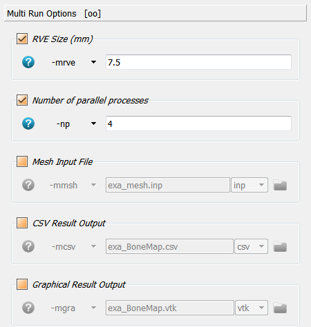
Click on * Multi Run Option* and activate the option -mrve for a multi-run
analysis (morhometric mapping). The parameter is the size of the reference volume
element (RVE) in mm. The distance between the RVE is set to half of this size
(50% overlap). The -np option is also actived to speed up the analysis
(multi-processing).
If this script is run, analyzes are performed but no result data is written. The
-mcsv options allows to output results in CSV format (readable by spreadsheet software
like Excel). The Script Output shows in this case:
... write CSV grid data    : Tb_Th
... write CSV grid data    : BVTV
... write CSV grid data    : BSBV
A typical CSV file contains:
#ElementId;Tb_Th_stddev;Tb_Th_mean
# min;0.076147478970677321;0.39199198078342229
# max;0.34801886170002377;1.1501820430063943
# mean;0.18064443569897159;0.74666198075560342
# std;0.035662715401958589;0.11575058763406647
1;0.20897835729369654;0.769512221789871
2;0.19088732119329496;0.78307305078656186
3;0.13252971283984724;0.55869138676742247
4;0.20049011599073643;0.82426653164838959
...
In the first line you will find the name of the data columns. The following commented out lines contain a simple statistical analysis of the data for each column.
The -mgra option activated the graphical output and the Script Output says:
... write VTK file         : exa_BoneMap_Grid_Tb_Th.vtk
    -> write POINT DATA Scalar  Tb_Th_stddev
    -> write POINT DATA Scalar  Tb_Th_mean
... write VTK grid data    : BVTV
... write VTK file         : exa_BoneMap_Grid_BVTV.vtk
    -> write POINT DATA Scalar  BVTV_smooth
    -> write POINT DATA Scalar  BVTV_voxel
... write VTK grid data    : BSBV
... write VTK file         : exa_BoneMap_Grid_BSBV.vtk
    -> write POINT DATA Scalar  BSBV_voxel
    -> write POINT DATA Scalar  BSBV_smooth
In this case, only (background) grid data was output. Visualizing the data with Paraview gives:
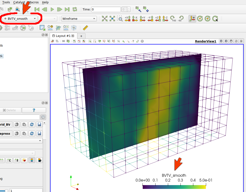
Note: There are usually more records in one VTK file. Therefore, it is important to select the correct record (see red mark in the picture).
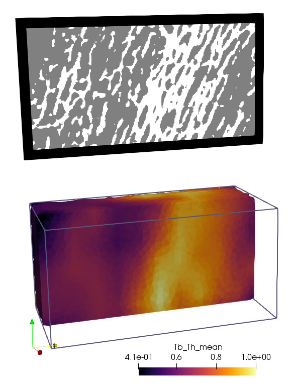
To map the data to a FE network, the option -mmsh needs to be activated. The
mesh from Step 3 (exa_mesh.inp) is inserted as input. For example, loading
the Tb_Th data in Paraview gives:
The Grid or FEM CSV data could be further processed as show in the example Grid Data Analysis.
Grid Data Scripting
Note
User Level: Expert
This example demonstrates the usage of several medtool’s libraries functions to read/write/create grid data (FEA mesh + results) for data analysis and visualizations.
In detail it demonstrates :
usage of medtool scripts as modules (library)
usage of user run script
read and write grid data files with fec class
generate and write FEA objects using dpFem class
generate and use of dpMesh class
The generated data files can be used for data analysis or visualization using e.g. Paraview.
Step 1
A user run script is created calling Extras - User Script Runner. A python script is given in the
-exe option using medtool’s python by writing:
python_medtool script.py
The GUI looks like:
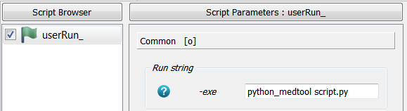
python_medtool is recognized by the User Script Runner and replaced by the locatation
where python was installed. The file script.py can be found inside the example folder.
If the working directory is not set to this example folder, the full path to script.py
has to be given which is done automatically by the medtool GUI).
Step 2
Open the file script.py with the Editor and explore the code. At the beginning libraries are loaded:
###  import libraries
import sys
import fec
where fec is a medtool library. If this script is not called with medtool, the PYTHONPATH
has to be set by the user.
After the import, a fec object is created:
myFec = fec.fec()
All implemented methods of fec (or myFec) can be shown by calling:
print help(myFec)
which gives the following information:
class fec
 |  Methods defined here:
 |
 |  __init__(self, modelName='default')
 |
  ...
 |
 |  readVTK(self, inFileName, results=False)
 |
  ...
 |
 |  write(self, outFileName, title, nodes, nsets, elems, elsets, NscaResults=None, EscaResults=None, vecResults=None, EvecResults=None, isBinary=False)
 |
  ...
The functions readVTK and write will be used in the following.
Step 3
In this step an existing data file (data.vtk) is read from the example folder using myFec:
print " read data file from disk"
print "-----------------------------------------------"
title, nodes, nsets, elems, elsets, NscaResults, EscaResults, \
                                    vecResults,  EvecResults = myFec.readVTK('data.vtk', results=True)
The data are read into variables (usually dictionaries). For example: :
nodes: is a Pythondictwith key=node_id and value=dpFem.node
elems: is a Pythondictwith key=element_id and value=dpFem.element
In order to check how a dpFem.node object is implemented one can write:
print help(nodes[1])
which returns the dpFem.node object with node_id=1 and shows:
class node
 |  Methods defined here:
 |
 |  __init__(self, id, x, y=None, z=None)
 |
 |  append_to_elemList(self, elementID)
 |
 |  get_coord(self)
 |
 |  get_coord_numpy(self)
 |
 |  get_dimension(self)
 |
 |  get_elemList(self)
 |
 |  get_id(self)
 |
 |  get_x(self)
 |
 |  get_y(self)
 |
 |  get_z(self)
 |
 |  set_coord(self, x, y, z)
 |
 |  set_coord_numpy(self, arr)
 |
 |  set_id(self, _id)
 |
 |  set_x(self, x)
 |
 |  set_y(self, y)
 |
 |  set_z(self, z)
 |
 |  show(self)
Writing the file to the disk is very similar to reading:
print " write data file to disk"
print "-----------------------------------------------"
myFec.write('exa_data.vtk', title, nodes, None, elems, None, NscaResults=NscaResults, EscaResults=EscaResults, \
                                                             vecResults=vecResults,   EvecResults=EvecResults)
The order and type of the arguments is the same as returned by the reading function.
The None means no nsets or elsets are passed which are not required for
vtk output. The write function is a generic functions which
detects the corresponding reader from the file extension.
This file can be viewed with Paraview (not included in medtool) and shows different type of elements as well as corresponding results (colours).
Step 4
Such data files can be also generated manually by the user. First, the data containers needs to be created which are dictionaries:
print " create dpFem objects manually "
print "-----------------------------------------------"

nodes       = {}        # node dict:      key = node Id,     value = dpfem node
elems       = {}        # element dict:   key = element Id,  value = dpfem element
nsets       = {}        # node set dict:  key = nset name,   value = node Ids
elsets      = {}        # elem set dict:  key = elset name,  value = elem Ids
Next, data objects are created and stored in the data container:
# ... create nodes
import dpFem # import medtool's dpFem library
noid=1; # arbitrary node id
x=0; y=0; z=0; # node coordinates
myNode = dpFem.node(noid,x,y,z) # create node object
nodes[noid] = myNode # add to dict with all nodes
noid=2; x=1; y=0; z=0; nodes[noid] = dpFem.node(noid,x,y,z)
noid=3; x=0; y=1; z=0; nodes[noid] = dpFem.node(noid,x,y,z)
# ... create element
elid = 1; # arbitrary element id
nList = [1,2,3]; # create a list, node connectivity
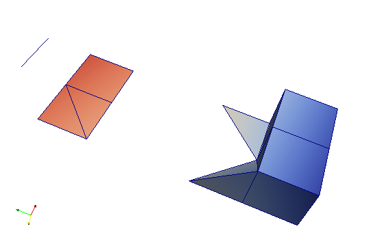
myElem = dpFem.element(elid, nList, 'tria3') # create 3-noded triangular element
elems[elid] = myElem # add to dict with all elements
# ... create element sets (important for ABAQUS, not vor VTK)
elsets["myElset"] = [] # arbitrary element set name
elsets["myElset"].append(elid) # append all element ids belonging to this set
In the first line the dpFem module is imported which defines dpFem.node, dpFem.elem, etc.
Next, required arguments are defined and the object (dpFem.node(noid,x,y,z)) is created.
In case of elements, many types are implemented (see Mesh- Converter -fec - documentation).
Step 5
Previously created object can be accessed with regular Python loops:
print " access dpFem objects "
print "-----------------------------------------------"
# ... loop over elements and print all node coordinates
for elid in elems :
  nList = elems[elid].get_nodes()
  print "  Elemend id = ", elid, "  Node Ids =", nList
  for nid in nList :
    print "     Node id = ", nid, "  Coords   =", nodes[nid].get_coord()
As mentioned above print help(nodes[nid]) shows all implemented methods of dpFem.node.
Also nodal (or point) and element (or cell) results can be added, respectively:
print " add node/element results "
print "-----------------------------------------------"
myNscaRes1 = {}                 # create dict for nodal scalar results
noid=1; myNscaRes1[noid] = 2.1  # add data for node Ids
noid=2; myNscaRes1[noid] = 3.7
noid=3; myNscaRes1[noid] = 8.5

myEscaRes1 = {}                 # create dict for first element results
myEscaRes1[elid] = 12.3         # add data for element Ids
myEscaRes2 = {}                 # create dict for another element results
myEscaRes2[elid] = -0.012
These mesh (or grid) with results can be written with:
print " write result file"
print "-----------------------------------------------"
myFec.write('exa_myData.vtk', "mesh", nodes, None, elems, None, NscaResults=[myNscaRes1], \
                                                     EscaResults=[myEscaRes1,myEscaRes2])
The nodes and elems variables give the grid of points and cells of the data file.
Looking in the output area of medtool it can be seen that following data are written:
 write result file
-----------------------------------------------
 ... write VTK file         :  exa_myData.vtk
     -> write POINT DATA Scalar: POINTScalar_1
     -> write CELL DATA Scalar: CELLScalar_1
     -> write CELL DATA Scalar: CELLScalar_2
i.e. one POINTScalar and two CELLScalar data are written.
Step 6
Finally, a mesh object form the dpMesh class is created from the previously define
nodes and element.
print " create a dpMesh (only trias!) "
print "-----------------------------------------------"
import dpMesh                                     # import medtool's dpMesh library
myMesh = dpMesh.dpMesh(nodes=nodes, elems=elems)  # create a dpMesh with nodes and elements from above
Note that dpMesh can only deal with triangles in 3D but it has a lot of useful
functions implemented e.g.:
print " explore dpMesh functions "
print "-----------------------------------------------"
print "   Element Area          :", myMesh.getElementArea(echo=False)
print "   Elements around Node  :", myMesh.getElementsAroundNode()
print "   Element Normal Vector :", myMesh.getNormalVector(elid)
which gives:
 explore dpMesh functions
-----------------------------------------------
   Element Area          : {1: 0.5}
   Elements around Node  : {1: [1], 2: [1], 3: [1]}
   Element Normal Vector : [ 0.  0.  1.]
Again all implemented methods of dpMesh can be listed with:
print help(dpMesh)
This example could be included into a medtool plugin to pass are arguments to the script and not hard-code them as done in here.
Grid Data Analysis
This tutorial shows how to use medtool’s grid data analyzer for multi-dimensional grid data analyses. The implementation is based on Pandas. Python Pandas data structures called ‘data frame’ are created. It is recommended to read the Pandas_in_10_min tutorial which is a short introduction to Pandas mainly for new users.
The input data files are generally data distributed in space, e.g. from finite element analyzes or from whole bone analyzes. In this case, an ID (element or node ID) is associated with each data point.
In this example you learn to:
read and manipulate grid data
re-group data
apply evaluations to obtain new data
visualize the grid data
The final medool database looks like this:
Step 1
In this step, we read and examine the data. Create from the menu Analyze - Grid Data
a script instance called _01_orig_gda. The data reader (option -inf)
recognizes the given pathname pattern according to the rules of a Unix shell
(* or ? wildcards). The specification of data*.xlsx lists and reads all files
from the working directory which show this pattern.
If you select the option -outs in the Data Output Options panel you get the
following output in the Script Output window:
         ELEM_ID   X1   X2   X3  VAR1  VAR2
data1 0        1  1.8  0.0  0.0    15   7.8
      1        3  0.0  2.6  0.0     9  -2.3
      2       10  0.1  0.2  3.4     4   3.5
data2 0        3  0.0  4.6  0.0    19 -12.3
      1        1  3.8  0.0  0.0    25  17.8
      2       10  1.1  2.2  5.4    14  13.5
data3 0        1  6.8  0.0  0.0    35  27.8
      1        3  0.0  7.6  0.0    29 -22.3
      2       10  3.1  4.2  8.4    24  23.5
The three data sets are automatically numbered (= index 0,1,2). There
variables ELEM_ID, X1, X2, X3, VAR1, and VAR2
are in the data frame.
Step 2
One can easily add further evaluations to the data frame by specifying formulas
using the -eval option within the Standard Computations tab. Creating a new script
called _02_eval_gda and setting the -eval to VAR3=VAR1+VAR2;VAR4=VAR1**2
gives:
         ELEM_ID   X1   X2   X3  VAR1  VAR2  VAR3  VAR4
data1 0        1  1.8  0.0  0.0    15   7.8  22.8   225
      1        3  0.0  2.6  0.0     9  -2.3   6.7    81
      2       10  0.1  0.2  3.4     4   3.5   7.5    16
data2 0        3  0.0  4.6  0.0    19 -12.3   6.7   361
      1        1  3.8  0.0  0.0    25  17.8  42.8   625
      2       10  1.1  2.2  5.4    14  13.5  27.5   196
data3 0        1  6.8  0.0  0.0    35  27.8  62.8  1225
      1        3  0.0  7.6  0.0    29 -22.3   6.7   841
      2       10  3.1  4.2  8.4    24  23.5  47.5   576
Use the -outi and -outi option within the Data Output Option panel
to write the input and output data frames to the disc, respectively.
xlsx and csv file formats are supported.
Step 3
Next we explore the re-group option by a new script called _03_regroup_gda.
First, set -index to ELEM_ID (switch the option -group and -fctn off)
within the Standard Computations tab.
This re-orders the data frame with respect to the ELEM_ID. Setting
-outs set to ON yields:
           X1   X2   X3  VAR1  VAR2
ELEM_ID
1        1.8  0.0  0.0    15   7.8
3        0.0  2.6  0.0     9  -2.3
10       0.1  0.2  3.4     4   3.5
3        0.0  4.6  0.0    19 -12.3
1        3.8  0.0  0.0    25  17.8
10       1.1  2.2  5.4    14  13.5
1        6.8  0.0  0.0    35  27.8
3        0.0  7.6  0.0    29 -22.3
10       3.1  4.2  8.4    24  23.5
Note: If this output is compared to the one of step 1, it becomes visible
that the 4th and 5th data line (file data2) have a different index.
The data are now indexed by ELEM_ID not by the row number.
Switching only -fctn on (switch off -group and -index) and using
the function mean gives:
ELEM_ID     4.666667
X1          1.855556
X2          2.377778
X3          1.911111
VAR1       19.333333
VAR2        6.333333
dtype: float64
The setting gives the mean of the whole dataset (all data files).
If -group and -fctn are actived ( -index is deactived) we
obtained:
     ELEM_ID        X1        X2        X3  VAR1       VAR2
0   1.666667  2.866667  1.533333  0.000000  23.0   7.766667
1   2.333333  1.266667  3.400000  0.000000  21.0  -2.266667
2  10.000000  1.433333  2.200000  5.733333  14.0  13.500000
This gives the mean of the data frame using the default index i.e. of
the data rows number. In this case the order of the data in the data files counts.
Finally, all three ptions - -group, -group, -index - are
activated which gives :
               X1        X2        X3  VAR1  VAR2
ELEM_ID
1        4.133333  0.000000  0.000000    25  17.8
3        0.000000  4.933333  0.000000    19 -12.3
10       1.433333  2.200000  5.733333    14  13.5
This gives the mean for the new index ELEM_ID. In other words, we
drilled through the record along the data files using the ELEM_ID variable.
In this case, however, the order of the lines or rows in the data file is irrelevant.
Step 4
In the last step, the data is displayed graphically. For this we create
the script _04_visualize_gda by clicking on Analyze - Grid Data again.
We keep the same settings as before (-group, -group, -index
are activated). The Mesh Output Option panel is modified in the
following way:
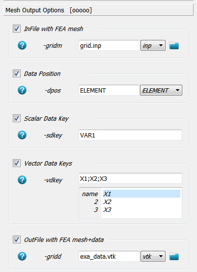
Shortly, a grid data file is given gridm called grid.inp which can
be viewed with the Editor. The data position -dpos is set to ELEMENT.
Scalar (-sdey) and vector data (-vdkey) are passed where the names
have to be in the data frame. The output is written to a file called
exa_data.vtk using the -gridd option.
The results can be viewed with Paraview after running this script. The final result can be seen in the following picture.
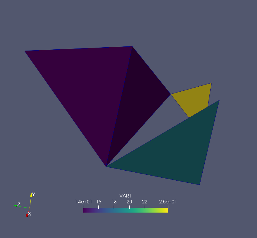
3D Printing from FE or Image
Note
User Level: Standard
This example shows how medtool creates 3D printable files based from medical 3D images (part 1 of this example) or from finite element model input (part 2).
Surface (STL) and voxel data files (mhd) are created, which are required for 3D printing on commercial devices.
In this example you learn to:
prepare a 3D image or FE Models to extract surfaces
extract surface meshes (stl) from segmented images
work with the interactive viewer in medtool
modify the extracted surfaces
explore the multi-material option
create printable files
The final medool database looks like this:
Step 1 (Part 1)
Create from the menu Image - Processor a script instance called mic_segment.
Select the file bone.mhd under (-in) option from the example folder, select as
output file exa_bone.mhd (-out option), and segment the image with the -thre0
option (‘70’ in this example). The image could be modified in any way. It is important
that finally a segmented image is written for the next processing step.
If you are not familiar with the Image - Processor, please work through the example
Image Processing first.
Step 2
Surfaces meshes can be done by clicking on Fabricate - 3d Print and create a new script
called fevox_image_1mat.
The previously generated segmented image is given with the -fin option (exa_bone.mhd).
Set the -show option ON to see the result graphically. After running the script, an
interactive window pops up. Simple interactions are possible. For example:
mouse functions: rotate (left hold), move (middle hold), or scale (right+hold)
F1 toggles the visibility of the surface model (initially ON)
F2 toggles the wire frame (initially OFF)
x,y,z toggles x,y,z cut. Use +/- to move the cut (initially OFF)
F7 makes screenshots
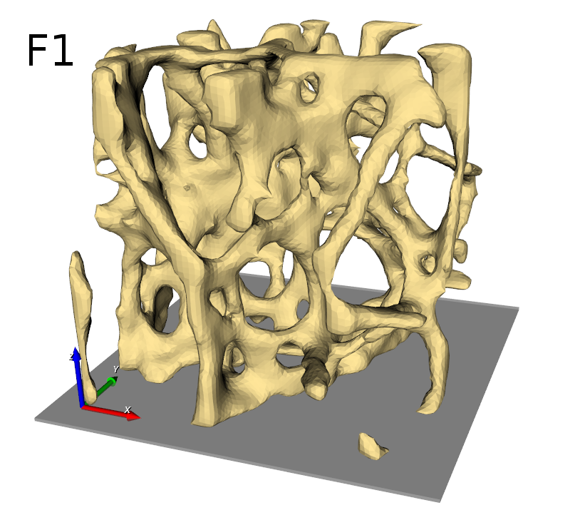
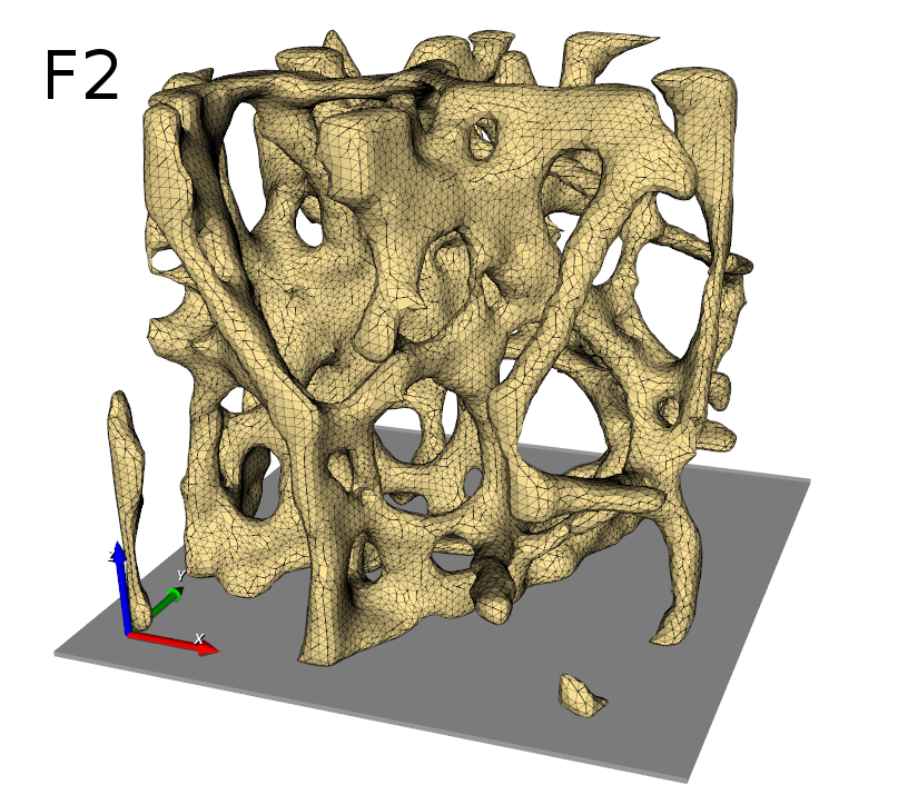
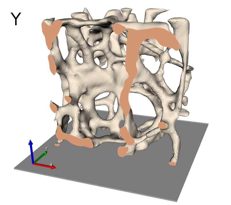
If -show is OFF all described process run in batch and do not need any user
interaction. In this way also medtool parameter studies can be done.
Step 3
Many options are available to modify the extracted surfaces using the Modify Image panel. More detail can be in the help of the script. Unique functions for stereolithography printers are the `` -stro`` options, which align the model so as to avoid breakage of the model during printing as well as the `` -conn`` options which removes unconnected regions (see figure below, left original surface, right corrected surface).
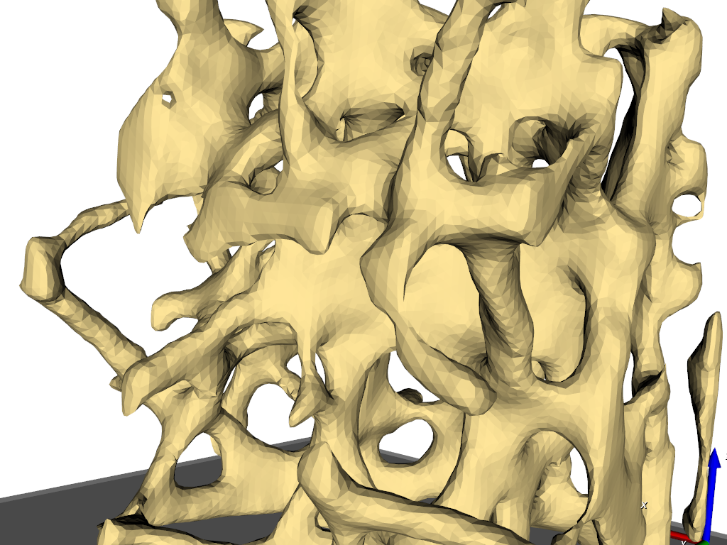
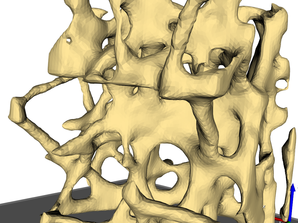
The Modify Surface panel contains typical surface modification options such as smoothing or decimating (see figure below, left original surface, right decimated surface by 50%).
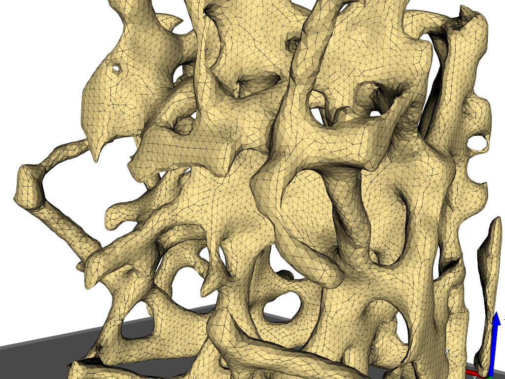
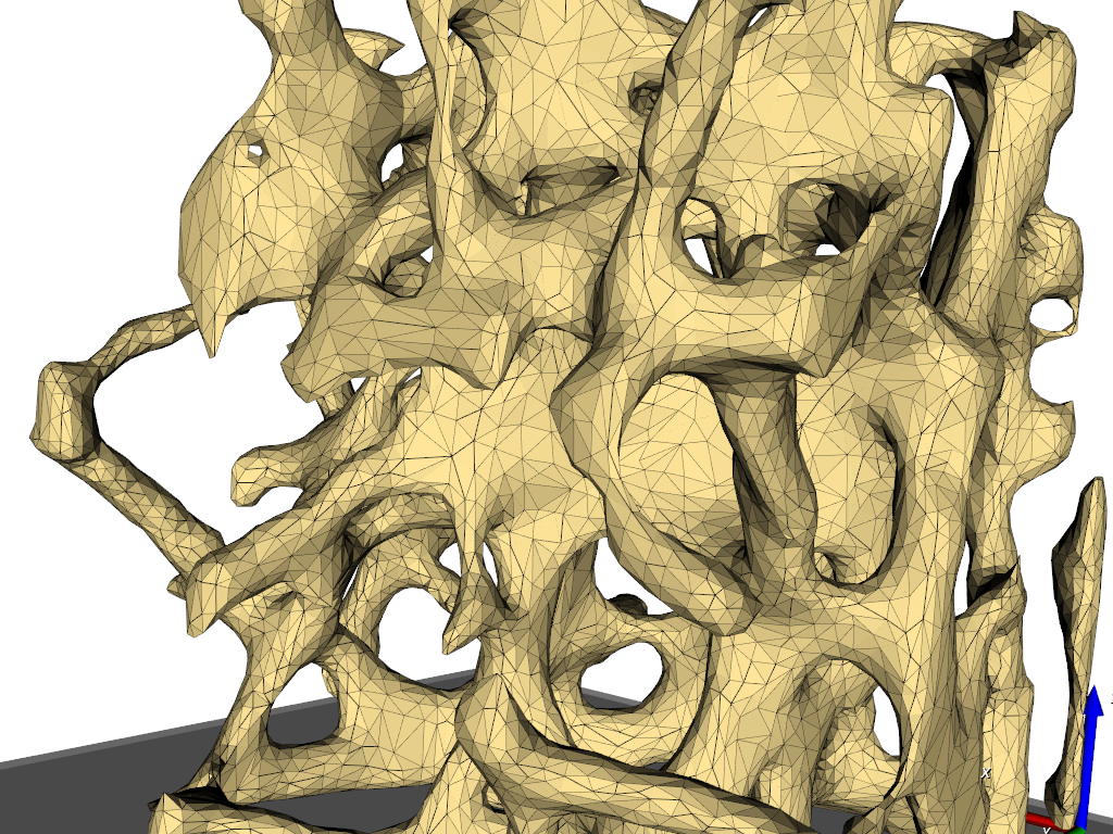
Inside the View Settings panel the style of the interactive view window can be changed. Useful are
the -cif and -cof options which can read or write camera postions. The file cameraPostition.txt inside
the example folder can be used to read a camera position with the -cif option. The following pictures
show the default view (left) and a view after reading a camera position (right):
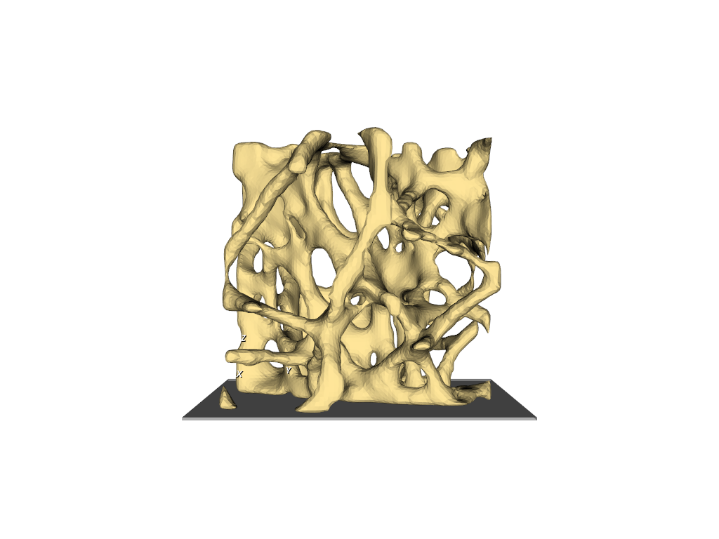
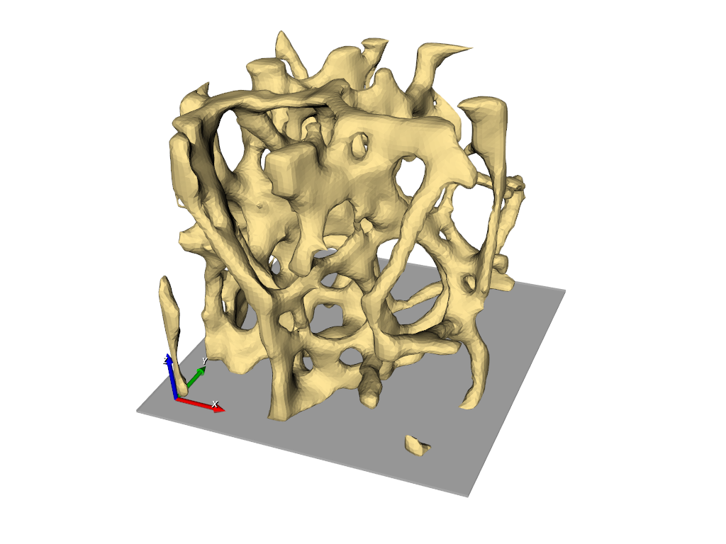
Step 4
The generated data can be written to several output formats. In general:
surface files can be written with
-outm(output mesh). These are STL, OBJ, or VMRL files.voxel based images can be written with
-outi(output image). E.g. the sapewayssvxformat but also images stacks likepngsand medical image formats likemhdornhdrare supported.screenshots can be written with
-screen. Additionally, three views are generated which can be read by the medool Viewer.
In this example the -outm option is used to write a file called exa_1mat.stl.
Step 5
In this step the -multi (multi material or gray-level) option is explored. Therefore, a second
Fabricate - 3d Print script called fevox_image_3mat is created. Select the file femur_3mat.mhd from
your example folder. This is a segmented image from the Image to Smooth Mesh (CGAL) example
showing three different gray values.
Next we switch -multi to ON and -axis to -z (Modify Image panel) to get the following output:
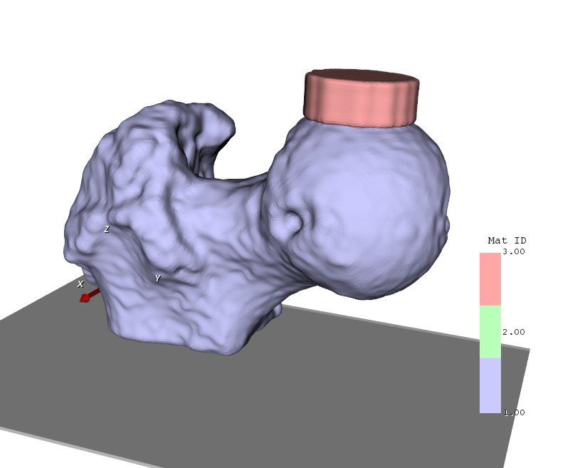
Three different material ids are identified. One for each gray-value. Finally, the surfaces are written with the
option -outm with the name exa_3mat.stl. Note that three stl files (one for each material id
exa_3mat_1.stl, exa_3mat_2.stl, exa_3mat_3.stl) are written.
Step 6
These three surface can be imported into a slicer software (e.g. Cura) to create the gcode file for a 3D printer. The image below shows such a slicing (left) and a make (right) where the outer shell is splitted into two pieces.
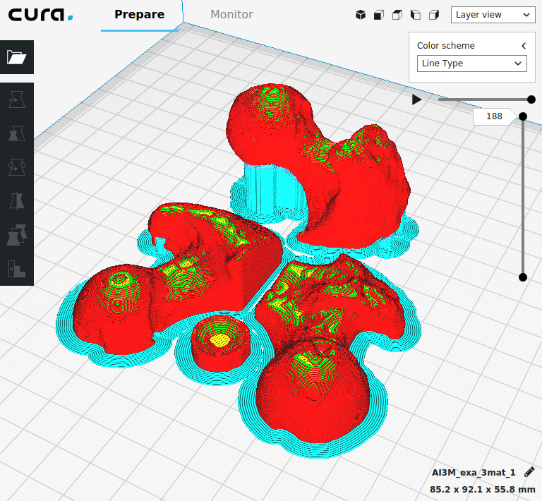
Step 1 (Part 2)
Alternatively, the Fabricate - 3d Print script allows Finite Elemente (FE) meshes as input.
Abaqus or Optistruct (Nastran) format is possible. A demo FE file (fe-model.inp) is located
inside the example folder. It can be opened and checked with the medtool Editor.
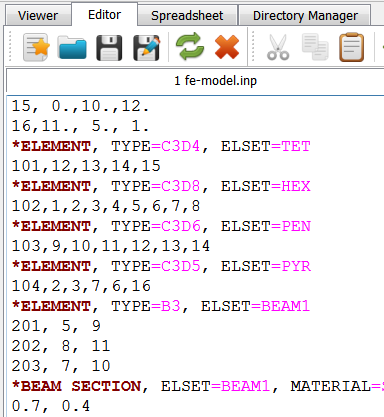
The geometry comes from the element type or in case beam or shell elements from the property definitions. Also the material ids are read by the script.
Step 2
An voxelizer script is created by clicking on Fabricate - 3d Print. After successful creation of the script, following options are edited inside the Common and FEA Parameters panel:
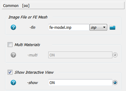
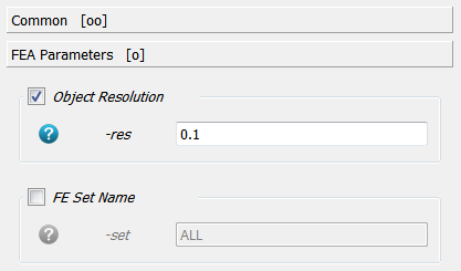
An FE file is selected (
fe-model.inp) using the-finoption. No path is given because the working directory was set accordingly as in the above examples.The resolution of the final voxelization have to be given and is chosen to be 0.1 mm (
-res) options. Based on this resolutions iso-surface are extracted using a discrete marching cube algorithm. This resolution could be similar to the resolution of the 3D printer. Higher resolutions provide more details but need longer computation times and produce larger output files.In order to see the voxelization the
-showoption is set toON. and an interactive render window pops up.
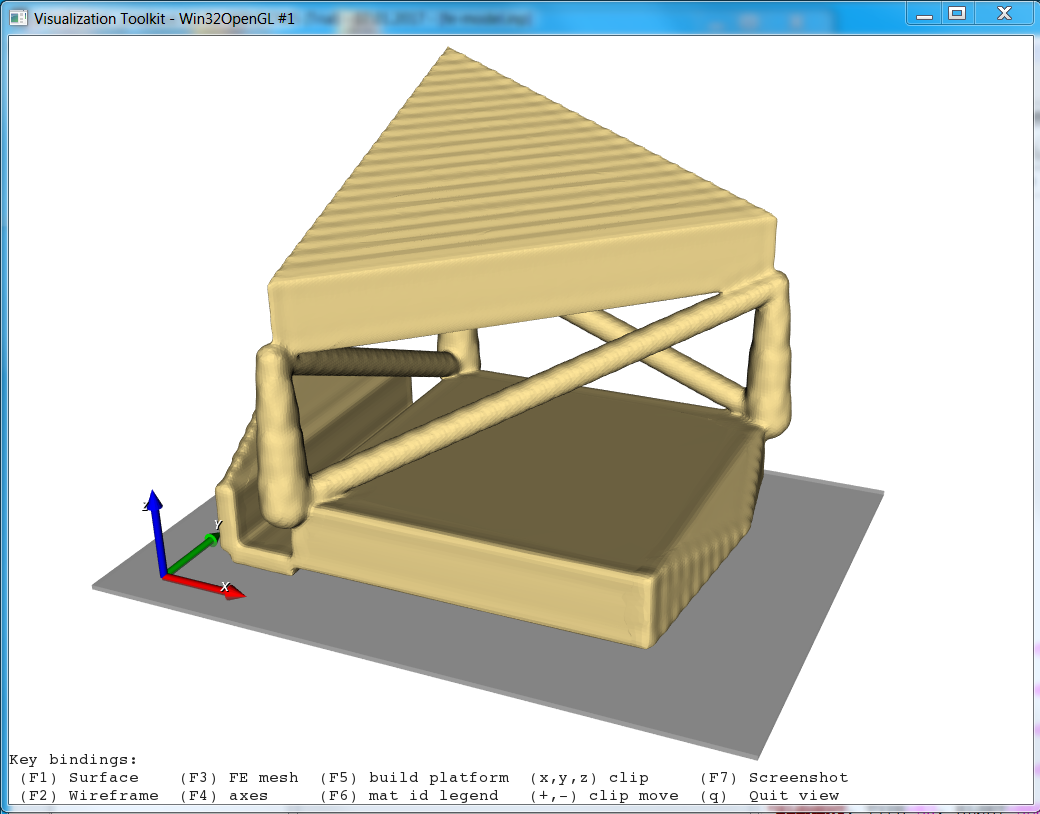
This view shows the build platform (gray) and the iso-surface which was extracted from the voxelized volume. The element size is roughly half of the resolution.
If -show is OFF all described process run in batch and do not need any user
interaction. In this way also medtool parameter studies can be done.
Step 3
The initial input and final results can be checked with the interactive window. Keys are used to interact with the window: For example:
F1 toggles the visibility of the surface model (initially ON)
F2 toggles the wire frame (initially OFF)
F3 toggles the visibility of the finite element model (initially OFF)
x,y,z toggles x,y,z cut. Use +/- to move the cut (initially OFF)
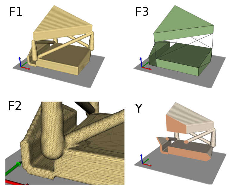
Step 4
Many modification are possible. For example, the option -set allows to process only individual
element sets or properties. Change -set to HEX;TET;PYR to extract
only elements with a material type ALU (see input deck) in the current example.
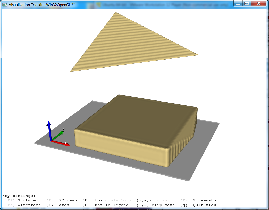
If the -multi option is set to ON than individual materials are colored starting with an id on 1. If this option
is ON a close surface is created for each material id. Otherwise a single closed surface is created.
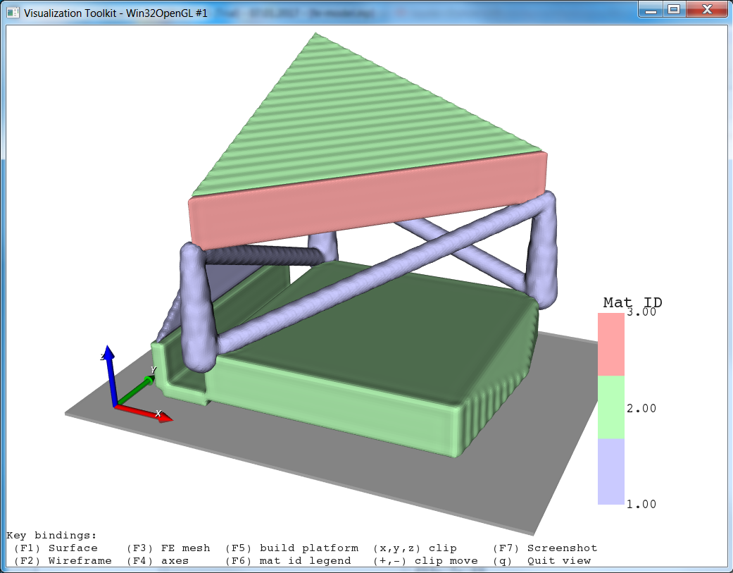
Inside the Modify Model panel many other things could be changed as described in more detail in the help. Shortly,
switch -multi to OFF and changing -axis to x (print direction) and the -decim to 0.9 (decimation of the surface mesh) gives (after showing the mesh with F2):
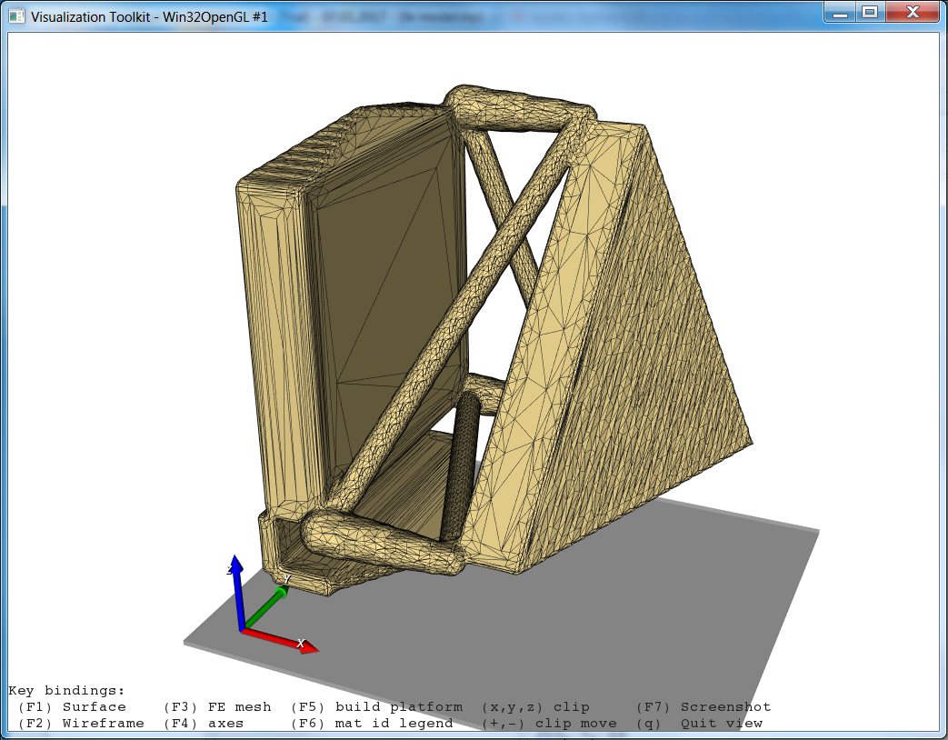
Inside the View Settings panel the style of the interactive view window can be changed. Useful are
the -cif and -cof options which can read or write camera postions. The file cameraPostition.txt inside
the example folder can be used to read a camera position with the -cif option. The following pictures
show the default view (left) and a view after reading a camera position (right):
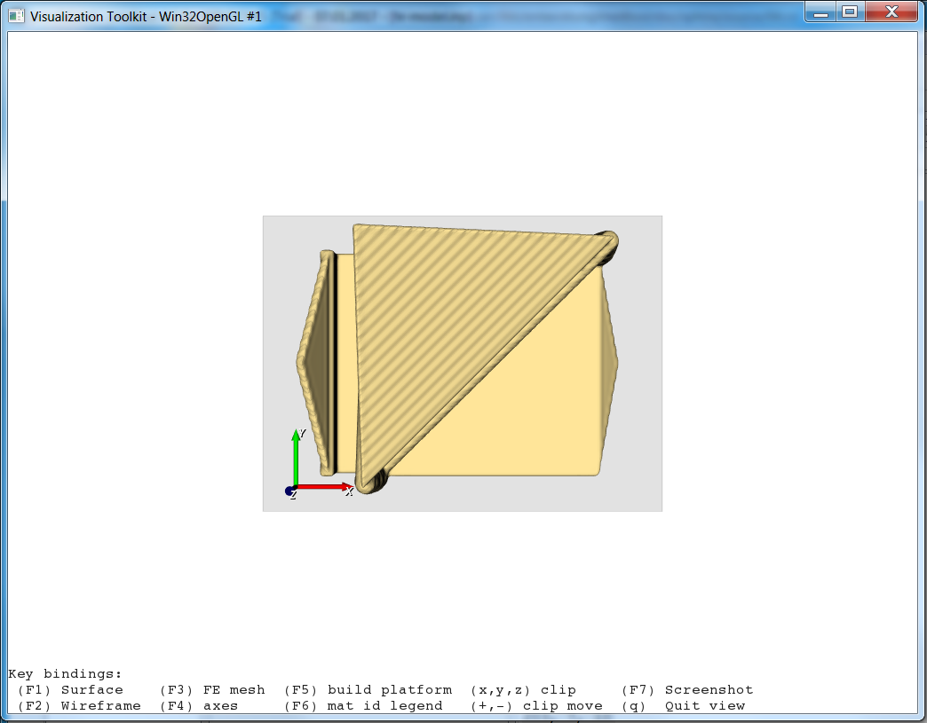
Step 5
The generated data can be written to several output formats. In general:
surface files can be written with
-outm(output mesh). These are STL, OBJ, or VMRL files.voxel based images can be written with
-outi(output image). E.g. the sapewayssvxformat but also images stacks likepngsand medical image formats likemhdornhdrare supported.screenshots can be written with
-screen. Additionally, three views are generated which can be read by the medool Viewer.
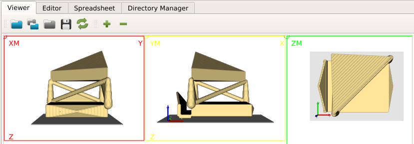
voxel based mid-planes can be written with the
-midoption.
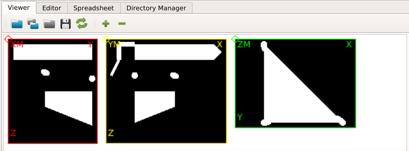
These data files could be directly used for printing. For example, an STL can be uploaded to shapeways which looks like:
Or sliced (e.g. using Cura) to print the model.
Simple ITK Integration
Note
User Level: Expert
This example explains the integration of Simple ITK in medtool. Python SITK libraries can be accessed via medtool’s Image - Processor script.
In this example you learn to:
convert between image formats
view images with matplotlib
segment images
register images
The final medool database looks like this:
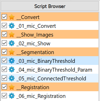
Step 1
In the first step, a file format is converted that is supported by SimpleITK
but not by medtool. Create from the menu Image - Processor a script instance
called _01_mic_Convert. Since no file is read via medtool, we write none
under -in option and write a midplane file to check the conversion
using the -mid option by specifying a file exa_brain_CT.png. Next switch
to the Simple ITK Filters panel and select the file ConvertImage.py in the
-sitkf option from the example folder. This filter allows to execute Simple
ITK code which is located in filename. The two variable names sitkInputImage
and sitkOutputImage are reserved for the input image and the output image,
respectively. The selected file contains the following Python code:
sitkOutputImage = sitk.ReadImage("training_001_ct.mha", sitk.sitkFloat32)
Remarks:
import SimpleITK as sitkis done automatically by medtool
sitkInputImageis not used in this examplethe output is written to the variable
sitkOutputImagean returned to the script
Step 2
In this step images are visualized with Python matplotlib and is based on this SimpleITK_matplotlib tutorial. The following sub steps are performed:
create an Image - Processor script called
_02_mic_Show
-inoption: select the filefemur-r8.mhdfrom the example folder
-sitkfoption: select the fileShowImage.pyfrom the example folder
This Python file contains two utility functions myshow and myshow3. The
main part of the file reads as:
# A) show single image
myshow(sitkInputImage, title="Femur")

# B) show single image label
img1_seg = sitk.BinaryThreshold(sitkInputImage, lowerThreshold=140)
myshow(sitk.LabelToRGB(img1_seg), title="Label Image as RGB")

# C) show multi images
size = sitkInputImage.GetSize()
myshow3d(sitkInputImage,yslices=range(30,size[1]-30,15), zslices=range(5,size[2]-5,15),  dpi=50)

# D) write medtool_ midplane images
mic.mic().writeMidplaneImages("exa_midplanes.png", sitk.GetArrayFromImage(sitkInputImage))

# E) give output image (is required)
sitkOutputImage = sitkInputImage
Point A) shows the input image sitkInputImage i.e. the z-midplane:
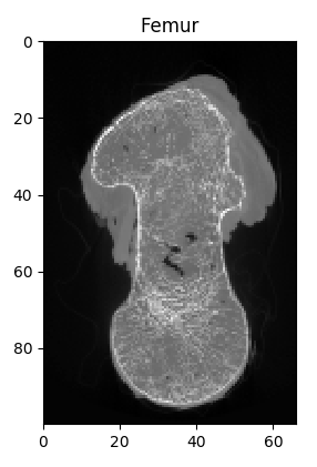
Point B) first the image is segmented and the colored label is shown as midplane:
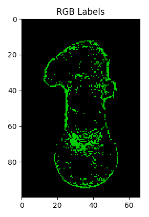
Point C) Multiple midplane images are shown.
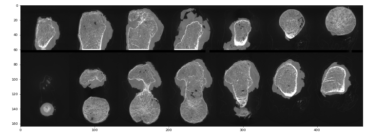
Point D) Also medtool midplanes can be written inside such Simple ITK scripts.
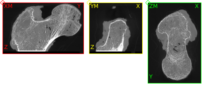
Point E) Finally, it is required to return an sitkOutputImage. In this case the
input is returned to the calling medtool script.
Step 3
A simple segmentation is carried out in this step. To do so:
-inoption: select the filefemur-r8.mhdfrom the example folder
-midoption: give a file nameexa_binaryThres.png
-sitkfoption: select the fileBinaryThreshold.pyfrom the example folder
This file contains the following python code:
sitkOutputImage = sitk.BinaryThreshold(sitkInputImage,
                                       lowerThreshold=140,
                                       upperThreshold=200,
                                       insideValue=255,
                                       outsideValue=0)
The following output is obtained (exa_binaryThres-XM.png):

Step 4
For parameter investigations, script parameter
must be passed to the Simple ITK script. This is done with option sitkp.
Similar to the above Step 3, the following steps are done:
-inoption: select the filefemur-r8.mhdfrom the example folder
-midoption: give a file nameexa_binaryThresParam.png
-sitkfoption: select the fileBinaryThreshold_Param.pyfrom the example folder
This file contains the following python code:
sitkOutputImage = sitk.BinaryThreshold(sitkInputImage,
                                       lowerThreshold=myLowerThreshold,
                                       upperThreshold=myUpperThreshold,
                                       insideValue=myInsideValue,
                                       outsideValue=myOutsideValue)
The parameter are transferred via the -sitkp option.
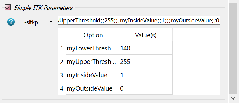
In the case of parameter runs, it is also possible to transfer parameters instead of values.
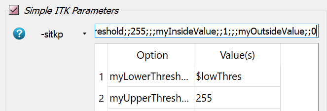
Step 5
In this example, a connected threshold with a seed is used. As before:
-inoption: select the filefemur-r8.mhdfrom the example folder
-midoption: give a file nameexa_connectThres.png
-sitkfoption: select the fileConnectedThreshold.pyfrom the example folder which
which contains:
sitkOutputImage =  sitk.ConnectedThreshold(sitkInputImage,
                                           seedList=[seed1],
                                           lower=lower,
                                           upper=upper,
                                           replaceValue=replaceValue)
First, a variable seed1 is specified in the seedlist.
It is also possible to specify several seeds i.e. seedlist=[seed1,seed2,seed3].
Seeds are simple obtained by the Image Viewer by:
open a midplane image
click on the location of a seed point (1)
go to the panel 2D Image Info (mouse click) and copy the value from the field Voxel Id i,j,k (2)
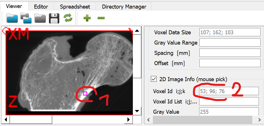
Copy this i,j,k values to the -sitkp option:
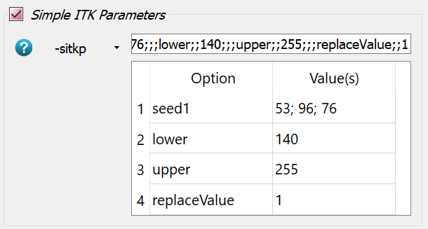
The difference between the binary threshold and connected threshold is show in the following figure:
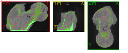
Step 6
This step shows a registration process of two images and is based on this SimpleITK_Registration example. Following steps are done:
-inoption: select as filenonebecause images are read by the Simple ITK script
-sitkfoption: select the fileRegistration.pyfrom the example folder
This script is very extensive and only the most important steps are explained and the resulting images are shown. First, images are read and displayed.
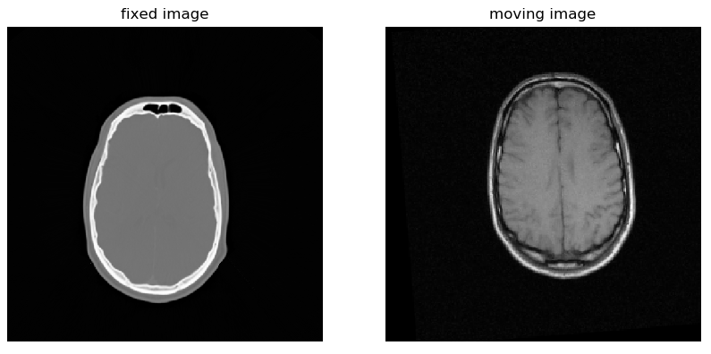
Second, images are initially aligned.
Third, the registration is executed and the metric is displayed.
Finally, the registration results are displayed
and the moving image is returned to medtool:
# Return final results to calling script
sitkOutputImage = moving_resampled
3D Slicer Bridge
Note
User Level: Standard
This example demonstrates the usage of a 3D Slicer extension to segment images manually. A view and ROI cut extension is also available. The medtool slicer bridge can be accessed via the Image - 3D Slicer script.
In this example you learn to:
The final medool database looks like this:
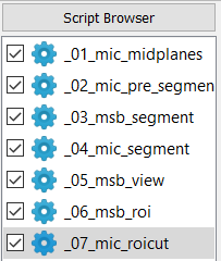
Step 1
In the first step, the content of the given file XR_image.mhd is viewed.
Create from the menu Image - Processor a script instance called _01_mic_midplanes.
Select this file in the -in option and write a midplane file exa_midplanes.png
to check the content.
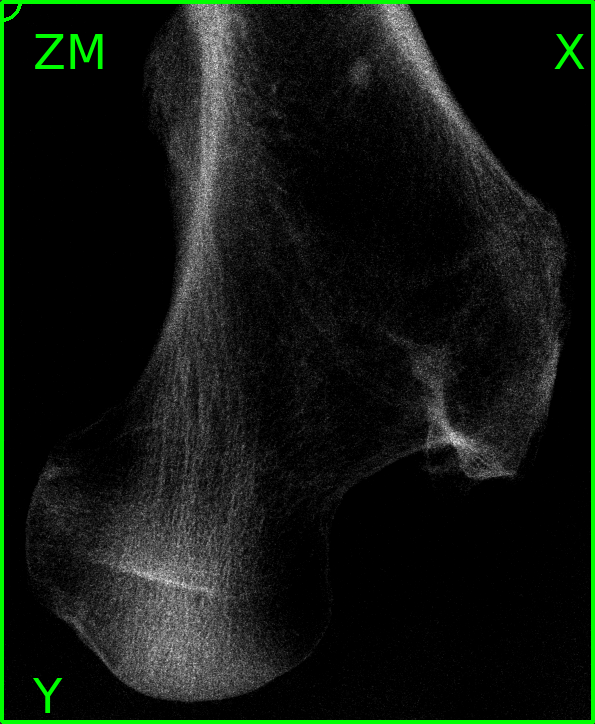
Step 2
Next, this image is roughly pre segmented using again a Image - Processor and applying a
-thre0 of 50. Don’t forget to write the file with -out option (file name
exa_pre_segment.mhd). The Viewer can be used to overlay this midplane with the previous image.
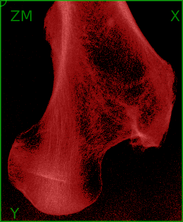
Step 3
In this step we take the pre-segmented images and further segment it interactively with 3D Slicer.
A medtool slicer bridge script is created by Image - 3D Slicer and denoted as
_03_msb_segment. Read the help of the script to get the basic idea behind the connection of medtool, Slicer extensions, and 3D Slicer. First
we set the original file XR_image.mhd as background images which helps to segment the boundary.
The -app option is set to segmentation. After that we click the Segmentation Option panel
in this script and set the -osg entry to exa_segment.mhd which holds the interactively segmented image.
In order to speed up the manual segmentation we pass also the pre-segmented image exa_pre_segment.mhd
from Step 2 via the -isg option to 3D Slicer. After clicking the Run Active button, a reduced 3D Slicer GUI is started.
Note
Before you can use 3D Slicer:
Install 3D Slicer (click on the link). 3D Slicer is not part of medtool and needs to be installed separately (medtool 4.5 works with version 4.11).
Open 3D Slicer without medtool and link all extension modules delivered with the medtool distribution (‘Slicer’ folder). This is done in 3D Slicer GUI under the menu ‘Edit’ - ‘Application Settings’ - ‘Modules’ - ‘Additional module paths’. It needs to be done for all extensions individually.
Install the ‘SegmentationEditorExtraEffects’ extension from ‘View’ - ‘Extension Manager’ menu.
Close 3D Slicer.
Set the 3D Slicer executable in medtool via Run Settings - 3D Slicer Executeable
Check the script Output panel to see if errors appear during start up.
The medtool - 3D Slicer bridge starts a reduced GUI which is shown in the following:
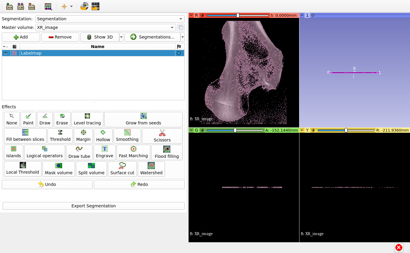
Select the Smooting tool and keep the default parameters.
Click Apply and the following image is obtained:
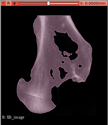
In the next step we use the Paint tool to close the holes. If you like you can smooth the resulting image again.
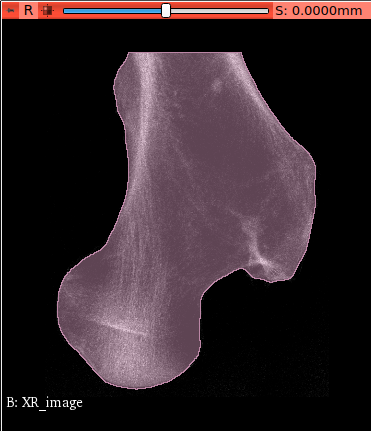
To finish up click the following button:
This saves the current segmentation in the file given in medtool to exa_segment.mhd. In case
you are repeating this procedure, you will be ask if you like to overwrite this file.
Note
Hide/Show full 3D Slicer view by clicking this button:
It allows to switch between the full and reduced 3D Slicer view.
After clicking the Back to medtool button, 3D Slicer will close an return to medtool. In case of a
parameter study, medtool will start the next script automatically.
Step 4
The midplanes of this segmentation can be further processed with medtool.
Simply an Image - Processor script _04_mic_segment is created and
the midplanes are viewed with -mid option.
Step 5
In this step we use the 3D Slicer bridge to view the segmentation by
creating an Image - 3D Slicer script called _05_msb_view. Perform
the following steps:
set the background image
-bvgto the original imageXR_image.mhdchange
-apptoviewgo to the View Options panel and
select as label map image
exa_segment.mhd(-lmvoption)start the script
This allows to overlay both images and inspect segmentations without modifying anything.
Step 6
To explore a further 3D Slicer bridge option, we crop a ROI from the
image. Create an Image - 3D Slicer script called _06_msb_roi.
Perform the following steps:
set the background image
-bvgto the original imageXR_image.mhdchange
-apptoroigo to the ROI Options panel and
select a text file
exa_roi.txt(-roioption) which stores the ROIstart the script
You see a ROI which can be manually changed in size. After you click
Back to medtool button, the file exa_roi.txt is saved.
Note
Look also at the 3D view (right) and check if the selected ROI is inside der image. Otherwise medtool throws an ‘outside image’ error.
Step 7
In this final step we crop the ROI by using the Image - Processor of
medtool. Create a script _07_mic_roicut and perform the following
steps:
set the input image
-into the original imageXR_image.mhdgo to the Resize Filters panel and
select the text file
exa_roi.txt(-roitxtoption) which contains the ROIwrite a midplane file with
-middenoted asexa_roi.pngstart the script
load and visualize the resulting midplane image
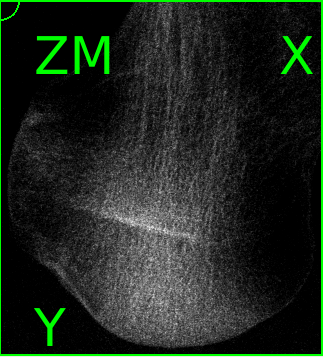
Image to microFEA
Note
User Level: Expert
This example demonstrates the usage of ParOSol and is very similar to the example Image to FEA. ParaOSol only runs on Linux and the post-processing requires Paraview.
The Image - Processor, Image - FEA Converter, Solve - Paraview, and Post - ParOSol scripts are used within this example. Five steps are done:
create a segmented image with end plates
generate an FEA model input deck for ParOSol
solving the model with ParOSol
creating an xmf file to read results in Paraview
post-processing the model with Paraview
The script browser has the following look for this example:
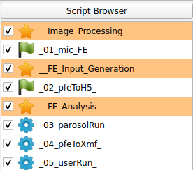
The entire workflow looks like this:
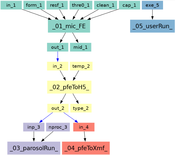
Recommendation: Work through the example Image Processing before you start with this one.
Step 1
This step is very similar to the step 1 of Image to FEA except that a fixed threshold (-thre0) is used
instead of -slevt. After all modifications, the image is exported as exa.mhd using the -out option.
Step 2
This labelled image is converted to an FEA input deck using Image - Converter FEA - ParOSol.
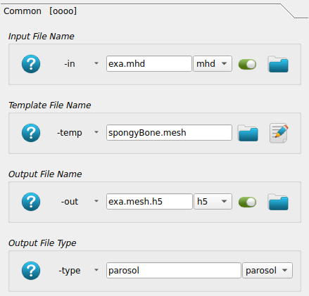
First, the input image FEA input deck exa.mhd is selected via -in.
Next a template file is loaded via -temp. The file spongeBone.mesh is provided in the
example folder and can be modified accordingly. This file looks like:
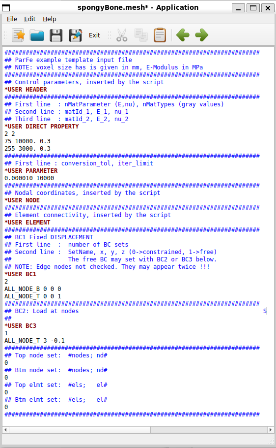
The variables of this script are used to created a *.h5 file. In more detail:
*USER DIRECT PROPERTYspecifies the material behavior: grayscale values of 75 represent bone, while grayscale values of 255 indicate embedding.
*USER NODEand*USER ELEMENTcreate the nodes and elements of the mesh.
*USER BC1specifies fixed displacement boundary conditions. The node setsALL_NODE_BandALL_NODE_Tare automatically generated internal node sets at the boundary surfaces.
*USER BC3specifies applied displacement boundary conditions. In this case, a -0.1 mm displacement is applied.
All other lines should remain as presented here.
The output is written to a file exa.mesh.h5 (-out) using parosol synthax (-type). This
is a HDF5 file format and could be also generate by hand, e.g. using the h5py library in python.
Note: Other versions of ParaOSol might use different input deck formats like ParOSolNL.
Step 3
In this step of the medtool script, an Finite Element analysis is performed using ParOSol.
This example is tiny and should run on any PC quickly (less than 1min). The interface to
ParOSol (Solve - ParOSol) needs the previously generate input file (exa.mesh.h5).
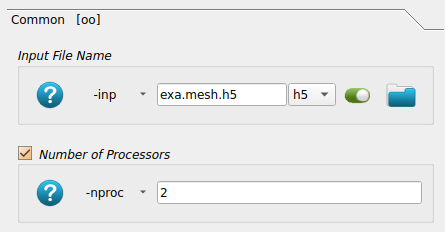
Only the number of processors is changed. ParOSol does not perform well for such small models and this is only an example. If the model is too small, ParOSol might crash. Usually micro FEA models are huge and need a lot of CPUs (nearly all CPUs of the maching).
The solution of the run is directly written into the exa.mesh.h5 under a
section Solution inside the file. Therefore, no output file is given.
Carefully check the messages on the Scrip Output area during the ParOSol run.
Step 4
In this step a file exa.mesh.xmf is created using (Post - ParOSol - H5 to XMF).
The xmf file is a meta data file and can be checked with the Editor.
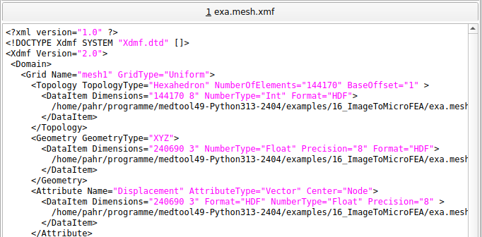
It contains the information needed by Paraview to read the exa.mesh.h5 file.
Step 5
Paraview (not included in medtool but it is freely available from https://www.paraview.org/) is started via Extras - User Script Runner to postprocess the results.
The standard xmf reader is selected to read the exa.mesh.xmf file
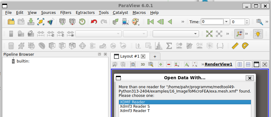
Typcial outputs are shown in the following. The displacments using the WarpByVector filter
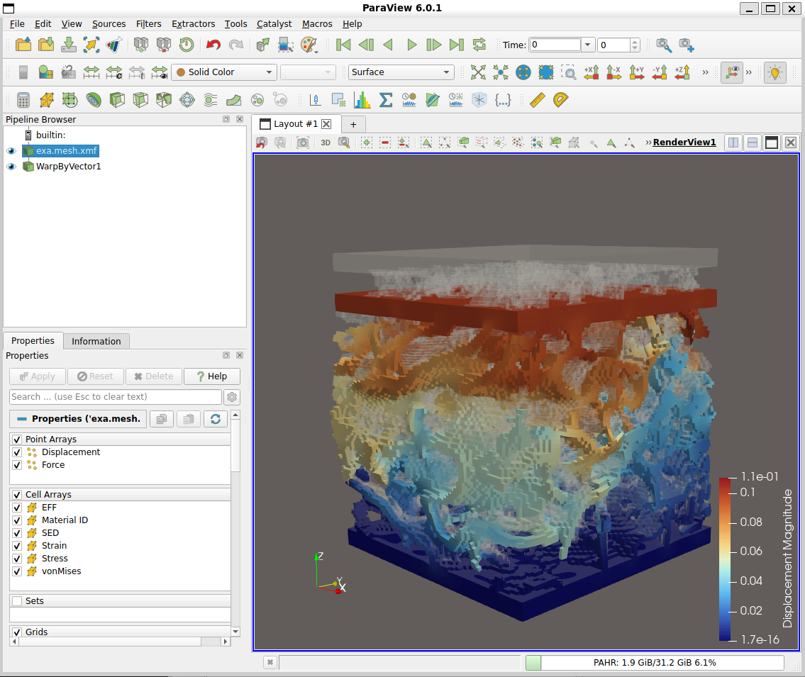
or the SED of a Clip filter.